One important characteristic of a microbiome community is its population diversity. The community diversity is highly related to its environment, so if a change of diversity has been detected, then it may either indicate that an environment in the human body has undergone a change (e.g., from a healthy to a disease condition) or indicate that the environment is disrupted by some factors (e.g., antibiotic use or a change of immune response). Thus, one task of microbiome community analysis is to find host and/or environment factors that can modulate the taxonomic composition (classified groups of closely related microbiota) and diversity (distribution of microbiota within or between communities) of the gut microbiota.
In microbiome community, generally there are three kinds of diversity including alpha, beta, and gamma diversities (Whittaker 1972). The alpha diversity and beta diversity are two common concepts that are used to measure the diversity of microbiome. In Chap. 9, we focus on alpha diversity analysis. Chapters 10 and 11 will introduce beta diversity analysis. This chapter is organized as follows. Section 9.1 introduces abundance-based alpha diversity metrics. Section 9.2 introduces phylogenetic metrics. Section 9.3 explores alpha diversity and abundance by some common plots. Section 9.4 describes statistical hypothesis testing of alpha diversity. Section 9.5 introduces alpha diversity analysis in QIIME 2. Finally, we briefly summarize this chapter in Sect. 9.6.
9.1 Abundance-Based Alpha Diversity Metrics
Although previously in the literature species diversity and species richness are sometimes used interchangeably, now it tends to use “species diversity” in the form of a species diversity index, that is, as an expression or index of some relation between number of species and number of individuals, and use “species richness” to refer to the number of species (in a given area or in a given sample) (Spellerberg and Fedor 2003).
Alpha diversity estimates the diversity within a single community (within-sample), which reflects both the number of species present (species richness) and the distribution of the number of organisms per species (species evenness), i.e., their relative abundance (evenness or equitability) and their taxonomic distribution. Several non-phylogenetic and phylogenetic metrics are available to measure alpha diversity. The non-phylogenetic metrics are based solely on abundance information, weight relatively rare, and mid-abundant and abundant species, while the phylogenetic metrics further utilize phylogenetic tree information.
9.1.1 Chao 1 Richness and Abundance-Based Coverage Estimator (ACE)
Species richness estimators estimate the total number of species present in a sample or community. Chao1 (Chao 1984) and ACE (abundance-based coverage estimator) (Chao and Lee 1992) were developed specifically for estimating richness of species from samples and for the general class-estimation problem, respectively (Colwell and Coddington 1994). In this section, we focus on Chao1 richness, and in Sect. 9.1.2, we introduce ACE.
9.1.1.1 The Measures of Chao 1 Richness
Two nonparametric methods of species richness for presence/absence data were developed by Anne Chao that were called “Chao 1” and “Chao 2” in the literature (Colwell and Coddington 1994). Chao1 index is a simple estimator to estimate the true number of species in the sample (or classes in a population) (Chao 1984); thus it is an abundance-based estimator of species richness.


Note that Chao index only uses the singletons and doubletons to estimate the number of missing species (Chao 1984) (see formula 9.1), so this index gives more weight to the low-abundance species. Therefore, Chao index is particularly useful for datasets skewed toward the low-abundance species (Hughes et al. 2001), as is likely to be the case with microbiome data.
However, from above formula, notice that if the number of singleton taxa n1 is getting larger, that is, a sample contains many singletons; in such case, it is likely that the sample exists more undetected species; then the Chao 1 index will estimate greater species richness than it would for a sample without rare species.

 This formula estimates the precision of Chao1 from multiple samples, replacing the more complex variance estimation technique presented in Chao (1984) (Colwell and Coddington 1994). The chao1 confidence interval for richness was developed in 2004 (Colwell et al. 2004).
9.1.1.2 The Measures of ACE

 is the estimated coefficient of variation for rare species (taxa, OTUs), which is defined as
![$$ {\gamma}_{\mathrm{ACE}}^2=\max \left[\frac{S_{\mathrm{rare}}}{C_{\mathrm{ACE}}}\frac{\sum_{i=1}^{10}i\left(i-1\right){n}_1}{N_{\mathrm{rare}}\left({N}_{\mathrm{rare}}-1\right)}-1,0\right]. $$](images/486056_1_En_9_Chapter_TeX_Equ5.png)
Chao and Yang (1993) discussed a theoretical optimal stopping rule based on the minimization of the testing cost and expected penalty due to the unremoved bugs. The optimal detection value is chosen as 10. The number of bugs detected more than 10 times is then added to the resulting estimate.
ACE method (see Eq. 9.4) divides the number of observed species into the frequencies abundant species (those with more than ten individuals in the sample) and the frequencies rare species (those with fewer than ten individuals) (Kim et al. 2017). The ACE method has some properties (Chao and Lee 1992; Chao and Yang 1993; Hughes et al. 2001; Sornplang and Piyadeatsoontorn 2016; Kim et al. 2017): (1) it only considers the presence or absence information of abundant species because abundant species would be discovered anyway; (2) it does not require the exact frequencies for the abundant species; (3) it does require the exact frequencies for the rare species because the estimation of the number of missing species is based entirely on these rare species.
9.1.1.3 Calculating Chao 1 Richness and ACE Using Ampvis2 Package
In this section, we use both ampvis2 and microbiome packages to illustrate the alpha diversity calculations based on two datasets. The first example is breast cancer QTRT1 mouse gut data (Zhang et al. 2020). The second example is mouse gut microbiome we generated from raw sequencing using QIIME 2 in Chap. 4 and has been used for bioinformatic analysis in Chaps. 5 and 6.
Sun and her team in 2020 conducted a murine microbiome experiment to explore whether and how the enzyme queuosine (Q)-tRNA ribosyltransferase catalytic subunit 1 (QTRT1) affects tumorigenesis and the microbiome. Queuosine is a micronutrient from diet and microbiome. Transfer RNA (tRNA) Q-modifications occur specifically in four cellular tRNAs at the wobble anticodon position. Because the microbiome product queuine is required for its installation, so tRNA Q-modification in human cells depends on the gut microbiome. This study aims to (1) examine microbiome-dependent Q-tRNA modification and its impact on breast tumor growth and gene expression and (2) identify the mechanisms of tRNA Q-modification-dependent cellular phenotypes in vitro and in vivo. Single clones of complete QTRT1-knockout (KO) in human breast cancer MCF7 cells were generated. The Q-modification levels of the MCF7 wild-type (WT) and QTRT1-KO cells were measured using the standard APB gel method. In this study, 20 KO mice (n = 10 for each of before and post treatments) and 20 WT mice (n = 10 for each of before and post treatments) were investigated. DNA was extracted from fecal samples, and 16S rRNA gene V3–V4 variable regions were barcoded and sequenced using MiSeq according to the Illumina protocol. After DNA sequencing, all possible raw paired-end reads were evaluated and merged using the PEAR (Zhang et al. 2014). Quality-filtered sequences were performed using QIIME pipeline (Caporaso et al. 2010) at a 97% similarity threshold utilizing the USEARCH algorithm (Edgar 2010) and the reference database silva_132_16S.97 (Glöckner et al. 2017). The microbiome data for downstream analysis include a total of 40 samples across 20 mice, resulting in 635 unique OTUs/taxa. The OTUs ranged from 39,813 to 65,762 for the individual sample, with a mean of 55,502.7 and median of 56, 093 and total reads of 2,220,108.
Throughout this book, we will call this dataset as “Breast cancer QTRT1 mouse gut microbiome” for simplification.
Because today most computers’ CPU can run eight processes simultaneously, thus unless you know your computer has a CPU with more (logical) cores than 8, setting it to 6 (Ncpus = 6) is a good starting point.
Windows users should also install Rtools4 on Windows. Starting with R 4.0.0 (released April 2020), R for Windows uses a toolchain bundle called rtools4 (https://mirrors.dotsrc.org/cran/bin/windows/Rtools/rtools40.html). Rtools4 is based on msys2, which makes easier to build and maintain R itself as well as the system libraries needed by R packages on Windows.
Here, we use breast cancer QTRT1 mouse gut data. The ampvis2 package can import data directly from the commonly used amplicon pipelines: QIIME 2, mothur, and UPARSE. The amp_import_biom() function is used to import the data in BIOM format generated from QIIME 2 and mothur, while the amp_import_uparse() function is used to import the data from the UPARSE pipeline. Then the data is loaded into a single ampvis2 object by the amp_load() function, which results in a list of data frames. The data that we use here are already in the format of data frames. Below we load otu_table and metadata into R:
Metadata variables: 4.
SampleID, Group, Time, Group4.
data is the required argument, listing as loaded with the amp_load() function.
measure is the listing vector that listed one or more alpha diversities to be calculated including “observed” for Observed taxa (OTUs), “shannon” for Shannon diversity, “simpson” for Simpson diversity, and “invsimpson” for inverse Simpson diversity.
richness is used to calculate sample richness estimates (Chao 1 and ACE) which is calculated by the estimate() function. The default is FALSE, without calculating richness.
rarefy rarefies species richness to the specified value before calculating alpha diversity and/or richness. By default(NULL), samples will be not rarefied before calculation.
9.1.1.4 Calculating Chao 1 Richness and ACE Using Microbiome Package
In order to show the workflow from bioinformatic data generation to downstream statistical analysis, here we use the same mouse gut microbiome data generated by DADA2 within QIIME 2. Thus we use qiime2R package to export the .qza and .tsv files into R. Entering the following R commands to install this package, then call the function qza_to_phyloseq() to create a phyloseq object. To do so, we also need the phyloseq package available:
9.1.2 Shannon Diversity
Shannon and Simpson diversity indices are most often used to measure the diversity of communities. Both indices take both abundance and relative abundances (evenness) of the species present into account. Thus they provide more information about the community composition than simple species richness (i.e., the number of species present).
9.1.2.1 The Measures of Shannon Diversity

 Thus, Shannon’s diversity index is to first calculate the proportion of species i relative to the total number of species (pi) and then multiplied by the natural logarithm of this proportion (lnpi). The resulting product is summed across species and multiplied by −1. In summary, Shannon’s index measures the uncertainty: How difficult would it be to predict correctly the species of the next individual collected? Put another way, it measures the amount of uncertainty, so that the larger the value of H, the greater the uncertainty.
Strictly speaking, the Shannon measure of information content should be used only on random samples drawn from a large community in which the total number of species is known (Pielou 1966).
Theoretically the value H could be very large because it increases as the number of species in the community increases and as the distribution of individuals among the species becomes even (Lemos et al. 2011; Magurran 2013). But in practice for biological communities, H does not seem to be larger than 5.0 (Washington 1984).
Shannon’s index “gives more importance” to less common categories (e.g., rare species in the case of microbiome) and places a greater weight on species richness than species evenness (Schloss and Handelsman 2006; Schloss et al. 2009).
Because Shannon’s index values increase as the number of sample size increases, thus normalization is crucial and suggested to avoid biases when it is compared between samples (Lemos et al. 2011).
Note that Shannon index is also known as the Shannon-Wiener index, the Shannon-Weaver index, and the Shannon entropy (Spellerberg and Fedor 2003). Based on Spellerberg and Fedor (2003), the uses of the “Shannon-Wiener” index and the “Shannon-Weaver” index are due to confusion. Actually, Shannon’s mathematical theory of communication including the first form of the present Shannon expression (index) was published in the 1948s Bell System Technical Journal (Shannon 1948). In 1949, Shannon published this information jointly with Warren Weaver, a mathematician, in the book The Mathematical Theory of Communication (Shannon et al. 1949), which is very similar to the original published papers, and the entropy “H” in 1948 was taken account of by Shannon in the first part of this 1949 book. In his paper Shannon appreciated the impact of the mathematician Norbert Wiener’s basic philosophy and theory on his communication theory and cited several of Wiener’s publications. Thus, Spellerberg and Fedor (2003) suggested that the “mislabeling” and the confusion of the Shannon index “H” (as referred to by Krebs 1999) as the Shannon and Weaver index are partly due to the joint authorship of Shannon and Weaver’s book, while given the fact that in the late 1940s, Shannon had built on the work of Wiener, it seems preferable to refer to “H” (the species diversity index) as the “Shannon index” or the “Shannon and Wiener index” (Spellerberg and Fedor 2003).
9.1.2.2 Calculating Shannon Diversity Using ampvis2 Package
The following R commands calculate Shannon index for QTRT1 dataset using the amp_alphadiv() in ampvis2 package:
9.1.2.3 Calculating Shannon Diversity Using Microbiome Package
To calculate Shannon diversity, we call the function alpha() in microbiome package and specify the index = “shannon”:
9.1.3 Simpson Diversity
Simpson’s diversity indices refer to four closely related indices: (1) Simpson’s index (D), (2) Simpson’s index of diversity 1 – D, (3) Simpson’s reciprocal index 1 / D, and (4) Simpson’s index of evenness.
9.1.3.1 The Measures of Simpson Diversity
Simpson in 1949 (Simpson 1949) proposed a new nonparametric measure which combines species richness and evenness. The new concept of diversity states that diversity is inversely related to “the probability that two individuals chosen at random and independently from the population will be found to belong to the same group” (Simpson 1949), i.e., will belong to the same species. Although in ecological literature the new concept of diversity is synonymous with diversity (Hurlbert 1971), it actually is about species heterogeneity (Good 1953).
Simpson’s index (D0) measures the probability that two individuals randomly selected from a sample will belong to the same species. This is Simpson’s original index, which is given as


This version of the formula will give consistent and acceptable results. In literature, Simpson’s original index in (9.7) is also written as  where S is the total number of species in the community and pi is the proportion of individuals (or relative abundance) of species i in the community. Simpson’s index gives more weight to the more abundant species in a sample. Additional rare species to a sample does not change the value of D0 too much.
The value of D0 ranges between 0 and 1, with 0 representing infinite diversity (i.e., the lower value of D0 the more diversity) and 1 suggesting no diversity (i.e., the bigger value of D0, the lower diversity). Obviously Simpson’s original index cannot provide an intuitive and logical interpretation of diversity.
To provide a straightforward interpretation, D0 is often subtracted from 1 which defines Simpson’s diversity index as below:

In the literature, Simpson’s diversity index is also written as  The values of Simpson’s diversity index also range from 0 to 1, but now with lower values (close to 0) indicating lower sample diversity, while greater values (close to 1) indicating greater sample diversity. Thus, Simpson’s diversity index measures the probability that two individuals randomly selected from a sample will belong to different species. In contrary to Shannon’s index, Simpson’s diversity index “gives more importance” to more common species.
Another way to avoid nonintuitive nature of Simpson’s index is to take the reciprocal of the index, which defines inverse Simpson’s index (1/D0). The inverse Simpson index is given as below:

As we stated above, heterogeneity contains both species richness and evenness; thus, researchers naturally try to separately measure the evenness component from richness. The null hypothesis of evenness is all species in a hypothetical community are equally common. However, most communities contain a few dominant species and many species that are relatively uncommon. Evenness measures attempt to quantify this unequal representation against the null hypothesis. As the independent measures of species richness, many different measures of evenness (or equitability) have been proposed in the ecology and microbiome literatures. Simpson’s index of evenness is one of them. Simpson’s index of evenness is obtained from reciprocal of Simpson’s original index  which is defined as

Simpson’s diversity index measures the species dominance and reflects the probability of two individuals that belong to the same species being randomly chosen. It varies from 0 to 1 and the index increases as the diversity decreases (Simpson 1949).
Simpson diversity puts a higher weight on species evenness more than species richness in its measurement (Schloss and Handelsman 2006; Schloss et al. 2009).
Same to Shannon diversity, normalization is considered as crucial and important to avoid biases when comparing Simpson diversity between different samples (Lemos et al. 2011).
9.1.3.2 Calculating Simpson Diversity and Inverse Simpson Diversity Using Ampvis2 Package
The following R commands calculate Simpson diversity for QTRT1 dataset using the amp_alphadiv() in ampvis2 package:
9.1.3.3 Calculating Simpson Diversity, Inverse Simpson Diversity, and Simpson Evenness Using Microbiome Package
To calculate Simpson diversity, we call the function alpha() and specify the index = “simpson” in the microbiome package:
9.1.4 Pielou’s Evenness
Pielou’s evenness (Pielou 1966) is the most common measure of evenness. Here, we describe and illustrate it below.
9.1.4.1 The Measures of Pielou’s Evenness

9.1.4.2 Calculating Pielou Evenness Using Microbiome Package
To calculate Pielou evenness, we call the function alpha() and specify the index = “pielou” in microbiome package:
9.2 Phylogenetic Alpha Diversity Metrics
Phylogenetic metrics not only use abundance information but also further utilize phylogenetic tree information. Several phylogenetic metrics are available to measure alpha diversity. In this subsection, we introduce three commonly used phylogenetic metrics: (1) phylogenetic diversity, (2) phylogenetic entropy, and (3) phylogenetic quadratic entropy.
9.2.1 Phylogenetic Diversity
Faith’s phylogenetic diversity (PD) (Faith 1992) is a measure of biodiversity, based on phylogeny (the tree of life), that is, incorporating phylogenetic difference between species. It can be considered as “a phylogenetic generalization of species richness” (Chao et al. 2016). Faith thought that the branch lengths on the tree are informative because they count the relative number of new features arising along that part of the tree. Thus, he defined and calculated the PD of a set of species as “equal to the sum of the lengths of all those branches that are members of the corresponding minimum spanning path” (Faith 1992), where “branch” is a segment of a cladogram, and the minimum spanning path is the minimum distance between the two nodes. The formula of PD is given as below:

9.2.2 Phylogenetic Entropy
Phylogenetic entropy (PE) (Allen et al. 2009) generalizes or extends the Shannon index (Shannon entropy) to incorporate phylogenetic distances among species. Thus, it is a diversity index (measure) that accounts for both phylogeny and species abundances, including species richness, evenness, and distinctness. The formula of PE is given as below:

Given defining PE this way, the Shannon index  becomes a special case of the PD if all species are equally distinct or, equivalently, if T has uniform branch lengths (Allen et al. 2009).
Shannon entropy does not obey the replication principle (or “doubling property”), which states that the total diversity of pooling two equally diverse and equally large groups with no shared species should be two times the diversity of a single group (Chao et al. 2010, 2016). PE (as a phylogenetic generalization of Shannon entropy) was reviewed having the same interpretational problem as Shannon index (Chao et al. 2010, 2016).
9.2.3 Phylogenetic Quadratic Entropy (PQE)
Phylogenetic quadratic entropy (PQE) (Rao 1982; Warwick and Clarke 1995), the most established quadratic diversity, measures the average taxonomic or phylogenetic distance between individual organisms. PQE that was introduced by Rao (1982) is a generalization of the Gini-Simpson index (Chao et al. 2016). It was independently rediscovered by Warwick and Clarke (1995) under the name “taxonomic diversity” (Allen et al. 2009; Warwick and Clarke 1995). The formula is given as below:

Although Rao’s quadratic entropy Q was the first diversity measure that accounts for both phylogeny and species abundances, however, like the Gini-Simpson index, its parent measure, it does not obey the replication principle. Thus it has the same interpretational problem as Gini-Simpson measure (Chao et al. 2010, 2016).
9.3 Exploring Alpha Diversity and Abundance
Alpha diversities and microbial abundances can be plotted using ampvis2 and microbiome packages. Comparing and visualizing groups based on the differences or similarities is also important. Various plots can be used to achieve different goals. We choose some useful plots to illustrate the capabilities of these two packages.
9.3.1 Heatmap
In this subsection, we illustrate how to generate heatmap using ampvis2 package.
The ampvis2 package generates plots using the ggplot2 package. The heatmap is generated by the amp_heatmap() function. This function by default aggregates data to phylum level and shows the top 10 phyla, ordered by mean read abundance across all samples. Before generating heatmap, let’s review a short summary of the breast cancer QTRT1 mouse gut data:
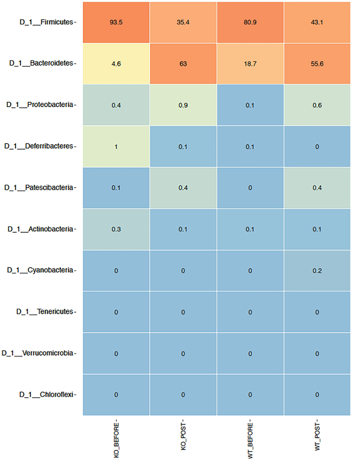
A heat map with different color gradients lists down the mean abundance value of Q T R T 1 gene data in the top 10 phyla at the phylum level. Firmicute ranks top in the heat map with values 93.5, 35.4, 80.9, and 43.1.
Heatmap of QTRT1 data aggregating to phylum level with the top 10 phyla, ordered by mean read abundance across all samples
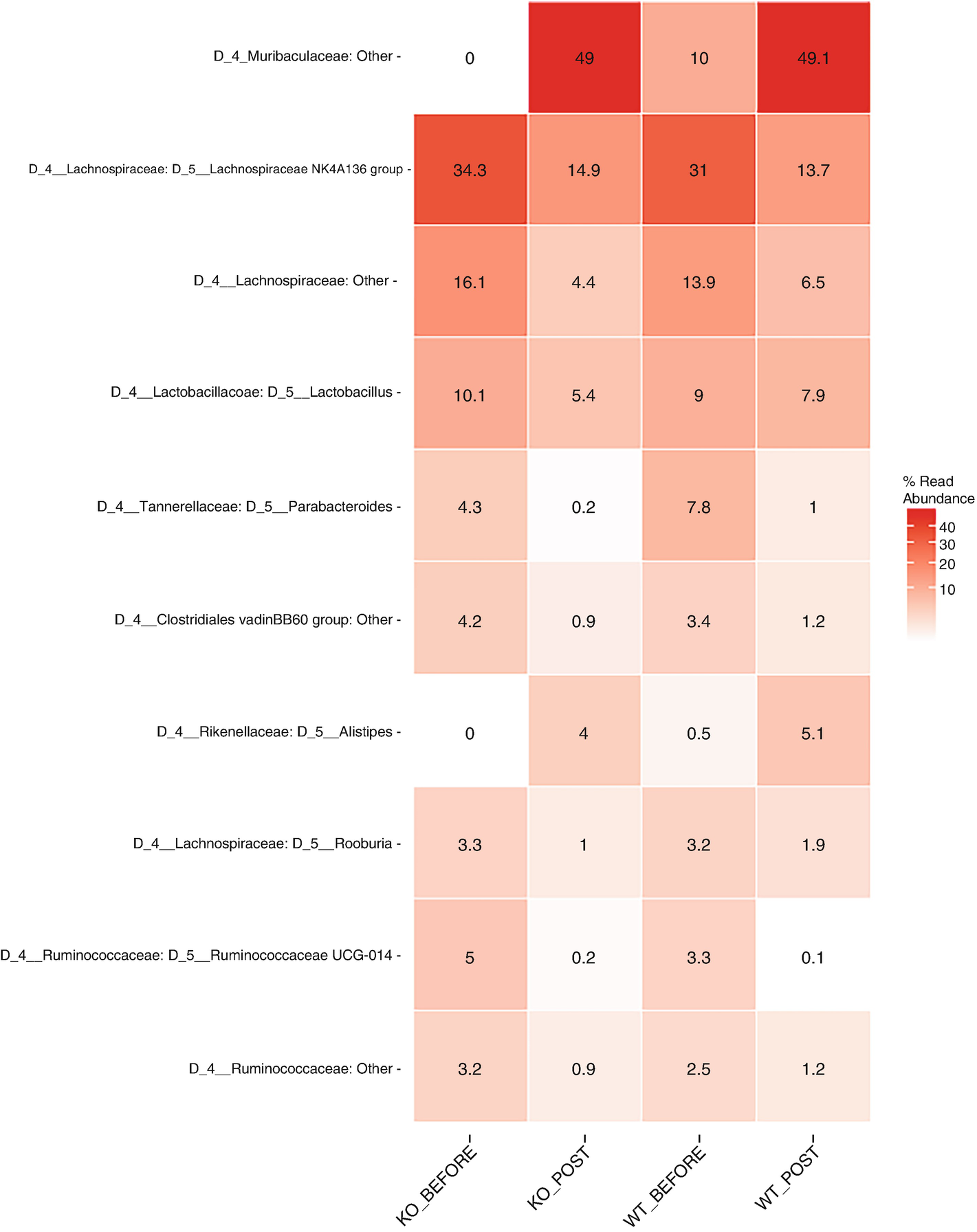
A heat map with different color gradients lists down the mean abundance value of Q T R T 1 gene data in the top 10 genera at the genus level. Muribaculaceae ranks top in the heat map with values 0, 49, 10, and 49.1.
Heatmap of QTRT1 data aggregating to genus level with the top 10 genera, ordered by mean read abundance across all samples
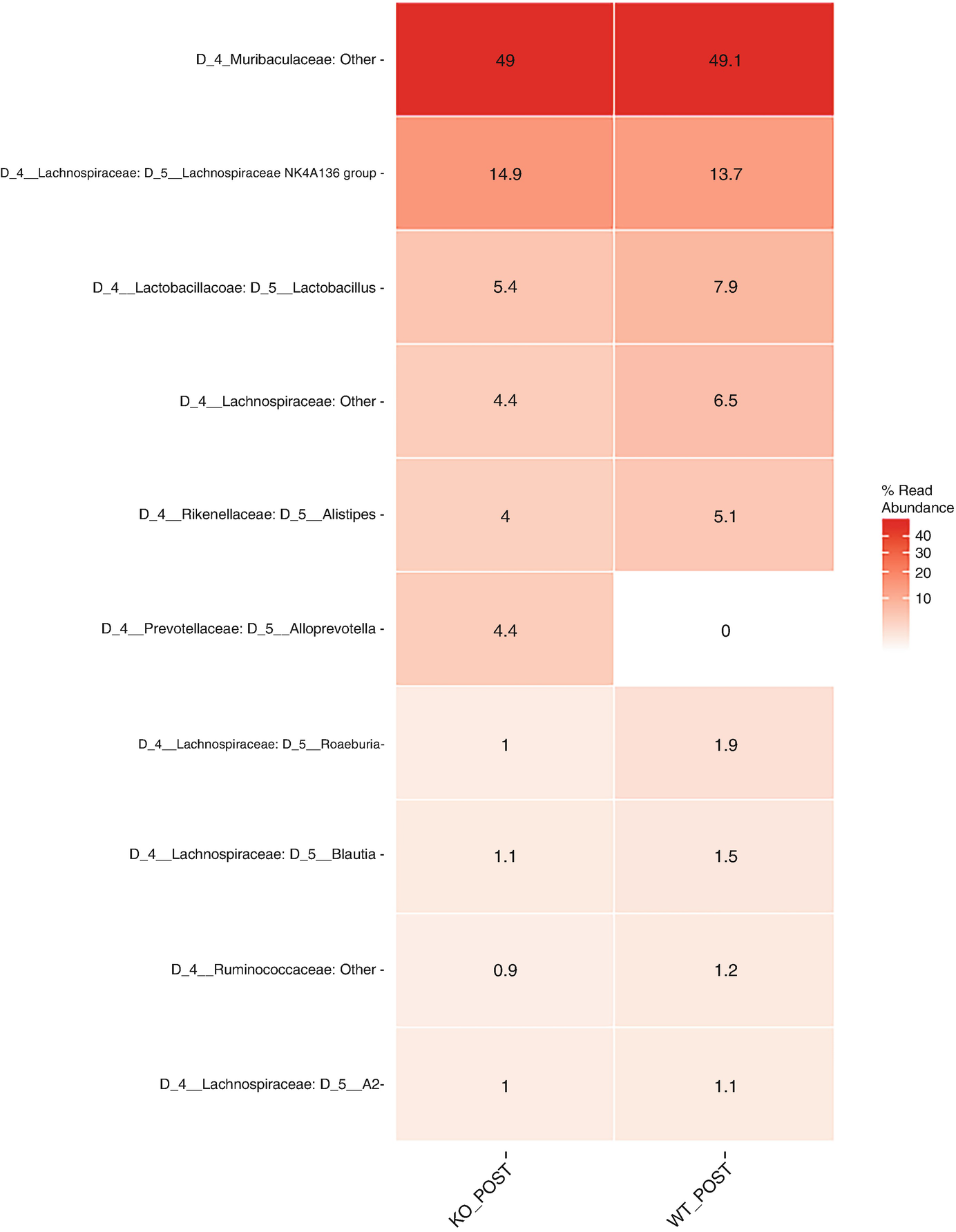
A heat map with different color gradients lists the mean abundance value of Q T R T 1 gene data in the top 10 genera at the genus level post-treatment. Muribaculaceae ranks top in the heat map with values 49 and 49.1.
Heatmap of QTRT1 data for post treatments aggregating to genus level with the top 10 genus, ordered by mean read abundance across all samples
We can subset the data based on two or more variables using “&” to separate the conditions or simply use the function more than once. The “!” (logical NOT operator) indicates “except” and is useful to remove outliers. The minreads = cut-off values argument removes any sample(s) with total amount of reads below the chosen threshold.
We can also subset the data based on the taxonomy using the amp_subset_taxa() function. For example, the following R commands subset the data to the taxa of D_3__Aminicenantales and D_3__Blastocatellales with a vector specifying their names separated by a comma:
9.3.2 Boxplot
In this subsection, we illustrate how to generate boxplot using ampvis2 and microbiome packages, respectively.
9.3.2.1 Generating Boxplot Using Ampvis2 Package
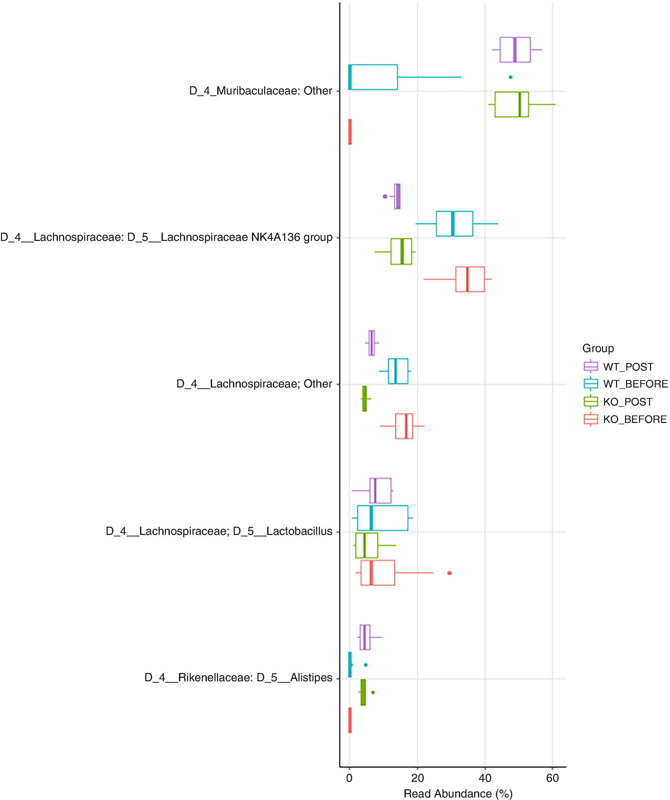
A boxplot of 5 different taxa versus real abundance in percentage. It displays data for the W T post and before and the K O post and before. W T post and K O post values are higher in Muribaculaeceae.
Boxplot of QTRT1 data for showing top 5 taxa with family information added
9.3.2.2 Generating Boxplot Using Microbiome Package
Next, we show steps to visualize the differences and/or similarities between groups using the microbiome package. By doing the plots, we need the useful R package ggpubr (current version 0.4.0, March 2022). The following R commands call the microbiome, ggpubr, and other two R packages:
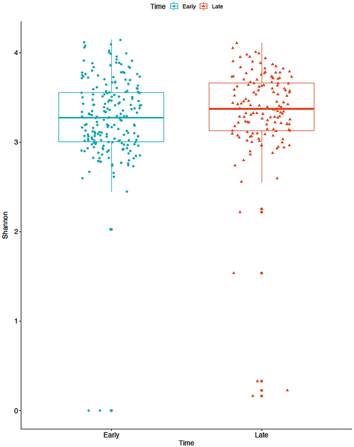
A boxplot of Shannon diversity of the gut microbiome measures the values at early and late time points as depicted by blue and red color boxplots. The values at the late time point are higher than at the early time point.
Boxplot of gut microbiome data for Shannon diversity by early and late time points in mice
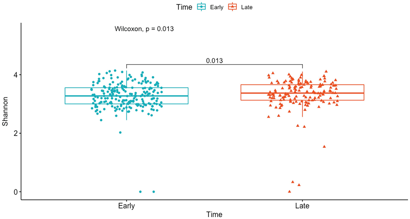
A boxplot represents Shannon diversity of the gut microbiome by p-values obtained at early and late time points of the Wilcoxon rank sum test. The p-value difference between the time points is 0.013 units.
Boxplot of mouse gut microbiome data for Shannon diversity by early and late time points with p-value generated by Wilcoxon rank sum test
Here the pairwise comparison P-value is the same as the global P-value because there are only two groups (early and late) in this comparison.
9.3.3 Violin Plot
For violin plot, we continue to use the same phyloseq object “physeq1” as in boxplot and compare differences in Shannon diversity between early and late time points.
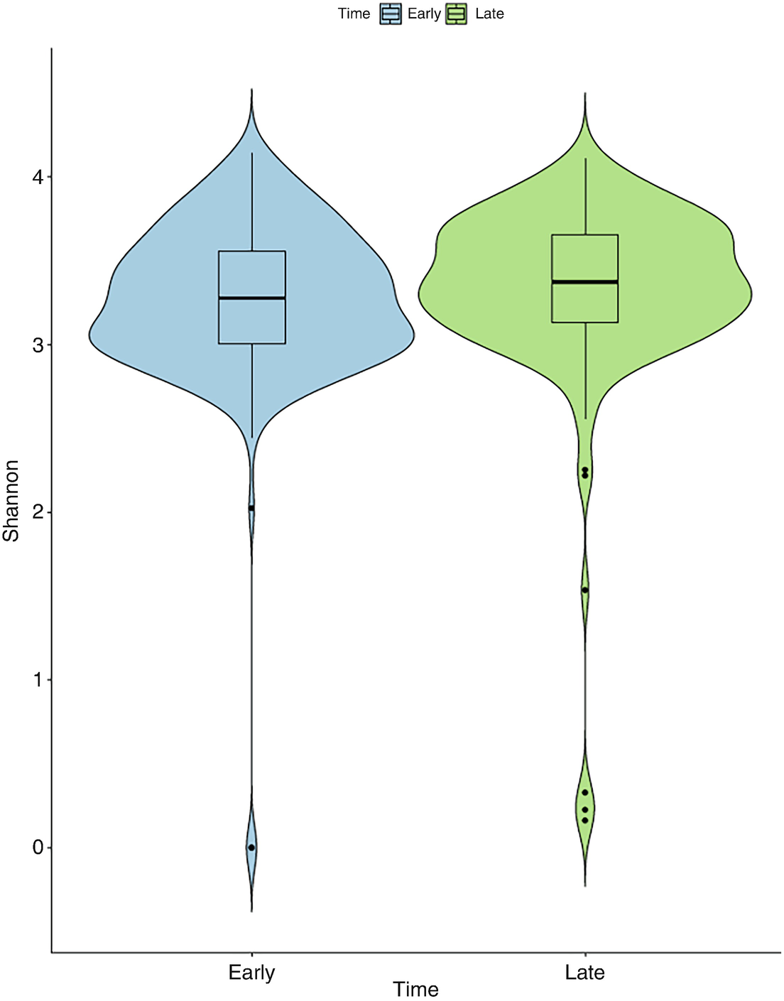
A violin plot of Shannon diversity of the gut microbiome measures the values at early and late time points as depicted by blue and green violin structures. The values at the late time point are broader than at the early time point.
Violin plot of mouse gut microbiome data for Shannon diversity by early and late time points
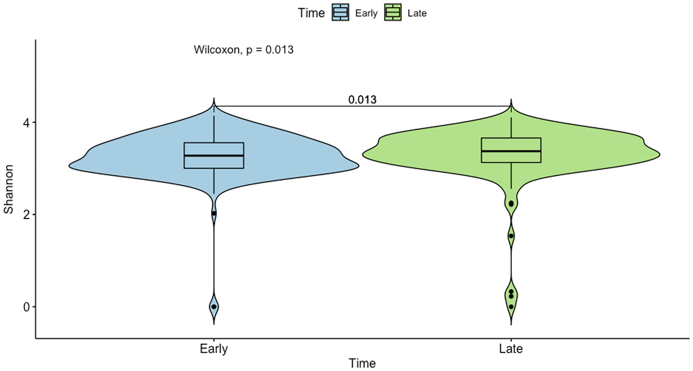
A violin plot of Shannon diversity of the gut microbiome measures the values at early and late time points as depicted by blue and green violin structures. The p-value difference between the time points is 0.013 units as measured by Wilcoxon sum test.
Violin plot of mouse gut microbiome data for Shannon diversity by early and late time points with p-value generated by Wilcoxon rank sum test
9.4 Statistical Hypothesis Testing of Alpha Diversity
Depending on the number of groups and the distribution of the alpha diversity measures, we can conduct a statistical hypothesis testing of alpha diversity using a two-sample Welch’s t-test, a Wilcoxon rank sum test, a one-way ANOVA, or a Kruskal-Wallis test (Xia et al. 2018). In above boxplots and violin plots, the P-values generated are from comparisons of Shannon diversity between early and late time points using Wilcoxon rank sum test. Here, we use the nonparametric Kruskal-Wallis test to compare groups (in the case of two groups, it equals to Wilcoxon rank sum test).
9.4.1 Summarize the Diversity Measures
9.4.2 Plot Histogram of the Diversity Distributions
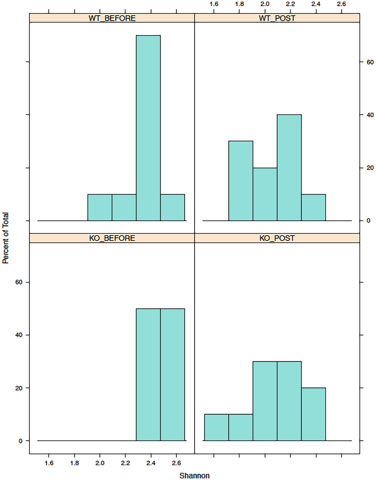
A histogram of the percent of total versus Shannon has 4 parts, W T before, W T post, K O before, and K O post. It displays that the highest values occur before the W T and K O parts.
Histograms of Shannon diversity in mouse gut microbiome data
9.4.3 Kruskal-Wallis Test
9.4.4 Perform Multiple Comparisons
Nemenyi’s test of multiple comparisons for independent samples (tukey).
9.5 Alpha Diversity Analysis in QIIME 2
QIIME 2’s diversity analyses are available through the q2-diversity plugin, which supports calculating alpha and beta diversity metrics, performing related statistical tests, and generating interactive visualizations. Both alpha and beta diversity measures, as well as phylogenetic and non-phylogenetic diversity measures, can be generated with a single command qiime diversity core-metrics-phylogenetic command. However, to show QIIME 2’s capabilities, in this section we will first use the core-metrics-phylogenetic command to calculate alpha and beta diversity metrics together, and then we will illustrate how to calculate each alpha diversity using individual alpha command. In Chap. 10, we will illustrate how to calculate each beta diversity using beta command. For diversity analysis, a sequence/feature/OTU table and a phylogenetic tree are required. And a sampling depth for random subsampling needs to be specified.
9.5.1 Calculate Alpha Diversity Using Core-Metrics-Phylogenetic Method
Here, we use a single command to generate all the phylogenetic and non-phylogenetic diversity measures available in QIIME 2. The alpha diversity measures calculated by the qiime diversity core-metrics-phylogenetic method include Shannon’s diversity, Pielou’s evenness, Faith’s phylogenetic diversity, and observed OTUs. The beta diversity measures calculated by this command include weighted/unweighted UniFrac (Lozupone and Knight 2005; Lozupone et al. 2007), Bray-Curtis, and Jaccard indices.
Because most diversity metrics are sensitive to different sampling depths across different samples, in order to compute samples with uneven sequencing depth, the core-metrics-phylogenetic method will randomly subsample or rarefy the counts from each sample to a user-specified value (i.e., sampling depth) when QIIME 2 computes these alpha and beta diversity metrics. Thus, it is crucial to provide the even sampling (i.e., rarefaction) depth to the parameter --p-sampling-depth. The algorithm works this way: The value provided to --p-sampling-depth will set up a total count for each sample in the resulting table when subsampling the counts in each sample without replacement. For example, suppose we specify 1000 for this parameter; then if the total count for any sample(s) are smaller than 1000, those samples will be dropped from the diversity analysis. The recommendation of choosing this value is to review the information presented in the Feature table.qzv QIIME 2 artifact and in particular the Interactive Sample Detail tab in that visualization. Typically, choose a value that is as high as possible (so that we can retain more sequences per sample) while excluding as few samples as possible.
Qiime tools view FeatureTableMiSeq_SOP.qzv.
Above command activates qiime 2 view. In the Interactive Sample Detail tab, we can see that sample M1D141 has 1153 sequences; then there are 10 samples from M3D8 to M3D149; the sequences decrease from 815, 694, … to the fewest sequence 0. Here we will choose 1153 based on the number of sequences in the sample M1D141. The value of 1153 is considerably or relatively higher than the number of sequences in the samples that have fewer sequences (from 694 to 0). Thus, choosing this value we can retain more sequences per sample while excluding few samples:
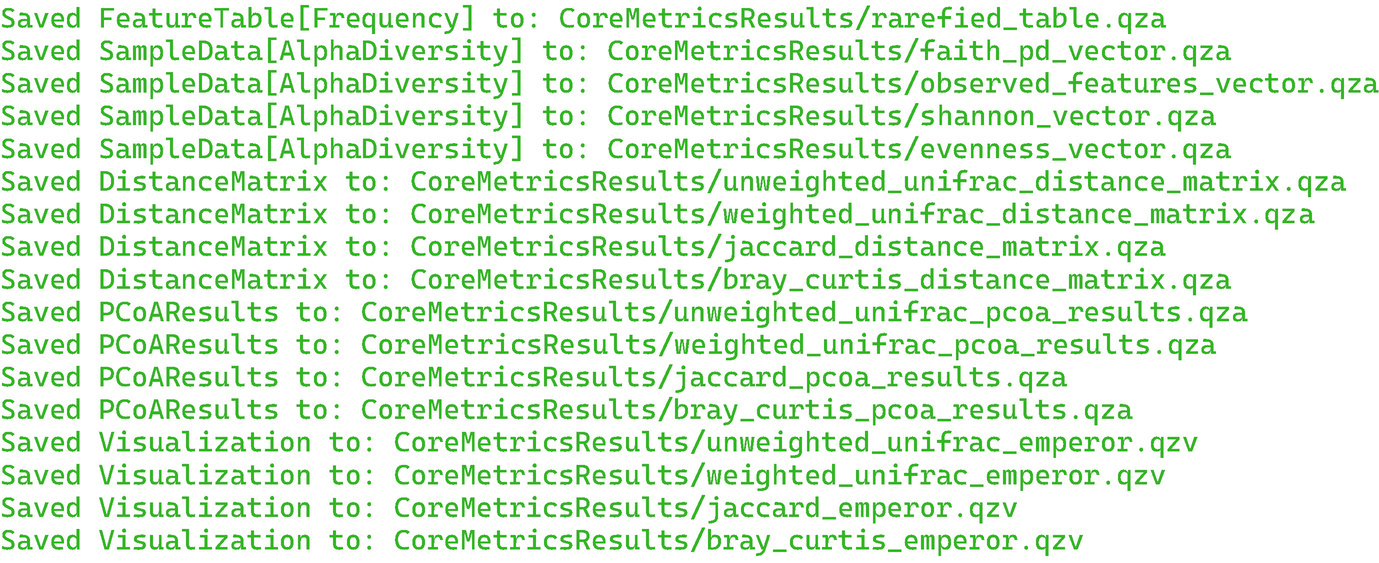
A set of 17 lines of data written in the green text represents the q z a format files saving locations.
9.5.2 Calculate Alpha Diversity Using Alpha Method
In QIIME 2, a user-specified alpha diversity metric for all samples in a feature table can be calculated using the alpha and alpha-phylogenetic methods for abundance-based (i.e., non-phylogenetic) alpha diversity metrics and phylogenetic alpha diversity metrics, respectively. Here, we continue to illustrate most frequently used abundance-based alpha diversity metrics using the mouse gut microbiome data in Example 9.12.
9.5.2.1 Shannon Index

A text reads, saved sample data, open bracket, Alpha diversity, closed bracket, to, S h a n n o n V e c t o r dot q z a.
The input parameter --i-table is used to specify the feature table containing the samples for which the alpha diversity metric will be calculated. The parameter --p-metric is used to specify the alpha diversity metric to be calculated. The output parameter --o-alpha-diversity is used to specify the output file, which you can give a meaningful name.
9.5.2.2 Chao1 Index and Chao1 Confidence Interval
The following commands calculate Chao 1 index which estimates diversity from abundant data and estimates number of rare taxa missed from under-sampling:

A text reads, saved sample data, open bracket, Alpha diversity, closed bracket, to, C h a o 1 V e c t o r dot q z a.

A text reads, saved sample data, open bracket, Alpha diversity, closed bracket, to, C h a o 1 C I V e c t o r dot q z a.
9.5.2.3 Observed Features
The following commands calculate observed features (here, OTUs):

A text reads, saved sample data, open bracket, Alpha diversity, closed bracket, to, O b s e r v e d f e a t u r e s v e c t o r dot q z a.
9.5.2.4 Simpson Index and Simpson’s Evenness

A text reads, saved sample data, open bracket, Alpha diversity, closed bracket, to, S i m p s o n v e c t o r dot q z a.

A text reads, saved sample data, open bracket, Alpha diversity, closed bracket, to, S i m p s o n E v e c t o r dot q z a.
9.5.2.5 Pielou’s Evenness

A text reads, saved sample data, open bracket, Alpha diversity, closed bracket, to, P i e l o u E v e c t o r dot q z a.
9.5.3 Calculate Alpha Diversity Using Alpha-Phylogenetic Method
QIIME 2 implements the phylogenetic alpha diversity metrics using the alpha-phylogenetic method.

A text reads, saved sample data, open bracket, Alpha diversity, closed bracket, to, F a i t h P D V e c t o r dot q z a.
The input parameter --i-phylogeny is used to specify the phylogenetic tree containing the tip identifiers that correspond to the feature identifiers in the table and is only used for the alpha-phylogenetic command for calculating phylogenetic diversity metrics.
9.5.4 Test for Differences of Alpha Diversity Between Groups

A text reads, saved visualization to, S h a n n o n G r o u p S i g n i f i c a n c e dot q z v.
The alpha-group-significance command generates boxplots of the alpha diversity values and runs all-group and pairwise Kruskal-Wallis tests, a nonparametric ANOVA to compare significant differences among all groups. We can activate qiime2.view to check the significant testing results. Three things are automatically done for each categorical data in metadata columns including alpha diversity boxplots, Kruskal-Wallis (all groups), and Kruskal-Wallis (pairwise). For example, for time variable, the results show that there are total 349 samples (208 for early and 141 for late times). Both all-group and pairwise Kruskal-Wallis show that later time has more Shannon diversity than early time with P-value of 0.003227 and Q-value of 0.003227. However, there is no difference of Shannon diversity between male and female mice with P-value of 0.826126 and Q-value of 0.826126. In this case, the results from all-group and pairwise Kruskal-Wallis are the same, and P-value is also equal to Q-value because the time variable only has two points. We can download the boxplots as SVG format or download raw data as TSV format. The Kruskal-Wallis testing results can be downloaded as CSV files.
The following commands conduct significant testing of Pielou’s evenness for all categorical variables in sample metadata:

A text reads, saved visualization to, E v e n n e s s G r o u p S i g n i f i c a n c e dot q z v.
The following commands conduct significant testing of Faith’s phylogenetic diversity for all categorical variables in sample metadata:

A text reads, saved visualization to, F a i t h P D G r o u p S i g n i f i c a n c e dot q z v.
The following commands conduct significant testing of observed OTUs for all categorical variables in sample metadata:

A text reads, saved visualization to, O b s e r v e d F e a t u r e s G r o u p S i g n i f i c a n c e dot q z v.
9.5.5 Alpha Rarefaction in QIIME 2
An alpha rarefaction analysis explores alpha diversity as a function of sampling depth, which is used to determine if an environment has been sequenced to a sufficient depth.
Alpha rarefaction is conducted by randomly subsampling the data at a series of sequence depths and plotting the alpha diversity metrics calculated from the random subsamples as a function of the sequencing depth. If a given sample has a plateau on the rarefaction curve, then it provides evidence that the sample has been sequenced to a sufficient depth to capture the majority of taxa.
In QIIME 2, we can use the qiime diversity alpha-rarefaction visualizer to conduct alpha rarefaction analysis. This visualizer will generate rarefaction curves using one or more alpha diversity metrics (by default based on Shannon diversity and observed features, i.e., OTUs measures) at multiple sampling depths, in steps between 1 (optionally controlled with --p-min-depth) and the value provided as --p-max-depth. In the case, if the phylogenetic tree is provided using the --i-phylogeny parameter, then this visualizer will also generate phylogenetic diversity-based curves.
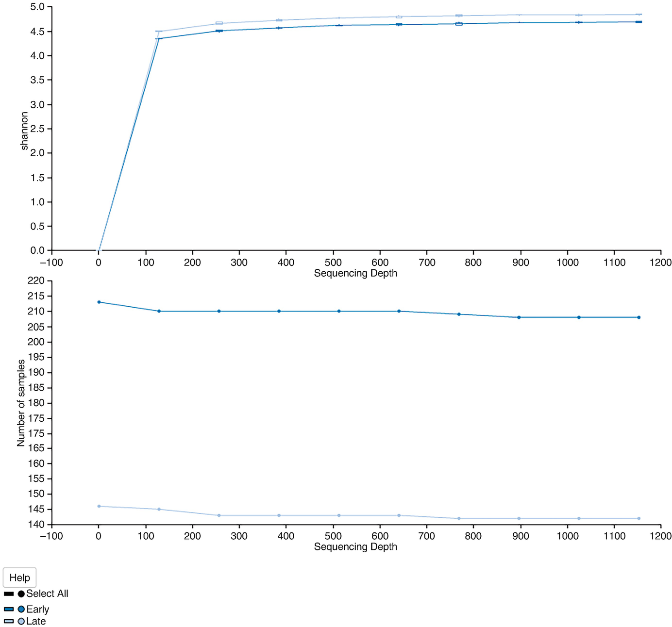
2 line graphs plot Shannon and the number of samples versus sequencing depth. Graph 1 displays 2 lines that increase gradually and become a plateau. Graph 2 exhibits 2 stable lines, one at the top and the other at the bottom.
The alpha rarefaction curves based on Shannon diversity with the results averaged by times

A text reads, saved visualization to, A l p h a R a r e f a c t i o n dot q z v.
The above command generates two plots. The alpha rarefaction plot at top is primarily used to determine if the richness of the samples has been fully observed or sequenced. If the slope of lines in the plot approaches zero or “level out” at some sampling depth along the x-axis, then it suggests collecting additional sequences (taxa) beyond that sampling depth likely to be either rare microorganism or the result of the sequencing error. In other words, the slope of lines does not approach zero; then it indicates either too few sequences were collected and thus the richness of the samples hasn’t been fully observed yet or the data remains having a lot of sequencing error; thus it is mistaken to use this data for diversity analysis.
The bottom plot is generated when sample metadata has grouping groups. It illustrates the number of samples that remain in each group when the feature table is rarefied to each sampling depth. The lines show the number of samples remains in each group when the feature table is rarefied to each sampling depth.
The essential function of the bottom plot is used to check whether the data presented in the top plot is reliable. Please note that we cannot specify a sampling depth that is larger than the total frequency that was obtained for a sample because it is impossible to calculate the diversity measure for this sample at the sampling depth.
Two patterns were noticed from this alpha rarefaction curve: One is that both early and late time points appear to plateau. The Shannon diversity measure does generally continue to increase as a function of the sequencing depth; however, the accumulation increases slowly, suggesting that we have sufficient sample sequence depth to have captured the majority of taxa present in the sample. Another pattern we can see from this plotting is that the late samples have a significantly higher Shannon diversity than the early time. This result is consistent with the Kruskal-Wallis test in Sect. 9.5.4.
9.6 Summary
In this chapter, we first introduced some most common used abundance-based alpha diversity measures and their calculations, including Chao 1 richness and abundance-based coverage estimator (ACE), Shannon diversity, Simpson diversity indices, Pielou’s evenness, and also three phylogenetic-based diversity measures: phylogenetic diversity (PD), phylogenetic entropy (PE), and phylogenetic quadratic entropy (PQE). We then illustrated three exploration tools for alpha diversity analysis: heatmap, boxplot, and violin plot. Next, we illustrated how to summarize and visualize alpha diversity measures and conduct statistical hypothesis testing of alpha diversity using Kruskal-Wallis test as well as perform multiple comparisons to adjust for P-values. Finally, we focused on alpha diversity analysis in QIIME 2 including how to (1) calculate alpha diversity using core-metrics-phylogenetic method, (2) calculate abundance-based alpha diversity using alpha method, (3) calculate Faith’s PD using alpha-phylogenetic method, (4) conduct statistical hypothesis testing of alpha diversity using Kruskal-Wallis test, and (5) perform multiple comparisons to adjust for P-values. We also illustrate how to generate alpha rarefaction curve in QIIME 2. In Chaps. 10 and 11, we will focus on investigating beta diversity analysis. In Chap. 10, we will introduce beta diversity metrics and their calculation using R and QIIME 2 as well as explore beta diversity using ordination methods. In Chap. 11, we will introduce statistical hypothesis testing of beta diversity.