12. Differential Abundance Analysis of Microbiome Data

12.1 Zero-Inflated Gaussian (ZIG) and Zero-Inflated Log-Normal (ZILN) Mixture Models

Both ZIG mixture and ZILN models are implemented in the metagenomeSeq package (Paulson 2020) via the functions fitZig() and fitFeatureModel(), respectively. The function fitZig() relies heavily on the limma package (Smyth 2005). The ZIG mixture was proposed first in 2013 (Paulson et al. 2013), which estimates the probability whether a zero for a particular feature in a sample is a technical zero or not. The fitFeatureModel() was later reparametrized to fit a zero-inflated model for each specific OTU separately. Currently the ZILN model along with the fitFeatureModel() is recommended (Paulson 2020).

The proposal of ZIG mixture model was motivated by the observation that the depth of coverage in a sample is directly related to how many features are detected in a sample. It was shown that there exist a relationship between depth of coverage and OTU identification ubiquitous in marker-gene survey datasets. Thus, ZIG mixture model was proposed to use a probability mass to accommodate the excess zero counts (both sampling zeros and structural zeros) and a Gaussian distribution to model the mean group abundance (the nonzero observed counts) for each taxonomic feature to explicitly account for biases in DAA resulting from under-sampling of the microbial community.

The model directly estimates the probability that an observed zero is generated from the detection distribution owing to under-sampling (sampling zeros) or due to absence of the taxonomic feature in the microbial community (structural zeros), i.e., from the count distribution. An expectation-maximization algorithm is used to estimate the expected value of latent component indicators based on sample sequencing depth of coverage.

The model is implemented via the metagenomeSeq package, mainly by implementing two methods: the cumulative sum scaling (CSS) normalization and zero-inflated Gaussian (ZIG) distribution mixture model.

The ZIG mixture model was designed to use the CSS normalization technique to correct the bias in the assessment of differential abundance (DA) introduced by total sum (TSS) normalization.

12.1.1 Total Sum Scaling (TSS)

In RNA-seq and microbiome literature, TSS (Paulson et al. 2013; Chen et al. 2018) and proportion (McMurdie and Holmes 2014; Weiss et al. 2017) are referred as the same method. TSS uses the total read counts for each sample as the size factors to estimate the library size or scale the matrix counts. TSS normalizes count data by dividing taxon or OTU read counts by the total number of reads in each sample to convert the counts to proportion.

Assume raw data is given as count matrix M(m, n), where m and n are the number of features (i.e., taxa, OTUs) and samples, respectively. Let counts c_ij represent the number of times taxonomic feature i was observed in sample j, the sum of counts for sample i is denoted as s_j = ∑_ic_ij, and then the normalized counts produced by the TSS normalization method is

(12.1)

At the beginning, microbiome researchers in practice simply used proportion or rarefying to normalize microbiome read counts. The proportion approach was directly adopted from RNA-seq field, while rarefying was inspired by the idea of rarefaction in ecology and hypergeometric model in RNA-seq data. In RNA-seq literature, TSS normalization has been evaluated to incorrectly bias differential abundance estimates (Bullard et al. 2010; Dillies et al. 2012) because a few genes could be sampled preferentially as sequencing yield increases in RNA-seq data derived through high-throughput technologies. For 16S rRNA-seq data, TSS or proportion also has been reviewed having limitations, including:

1. 1.

   TSS is not robust to outliers (Chen et al. 2018), is inefficient to address heteroscedasticity, is unable to address overdispersion, and results in a high rate of false positives in tests for species. This systematic bias increases the type I error rate even after correcting for multiple testing (McMurdie and Holmes 2014).

    
2. 2.

   TSS lies on the constant-sum constraint; hence it cannot remove compositionality; instead it is prone to create compositional effects, making nondifferential taxa or OTUs appear to be differential (Chen et al. 2018; Mandal et al. 2015; Tsilimigras and Fodor 2016; Morton et al. 2017).

    
3. 3.

   TSS has a poor performance in terms of both FDR control and statistical power at the same false-positive rate, compared to other scaling or size factor-based methods such as GMPR and RLE because of strong compositional effects (Chen et al. 2018).

    
4. 4.

   Actually, like to rarefying, TSS or proportion is built on the assumption that the individual gene or taxon count in each sample was randomly sampled from the reads in multiple samples. Thus, counts can be divided by total library size to convert to proportion, and gene expression analysis or taxon abundance analysis can be fitted via a Poisson distribution. Because in both RNA-seq data and 16S rRNA-seq data, the assumption cannot meet, the sample proportion approach is inappropriate for detection of differentially abundant species (McMurdie and Holmes 2014) and should not be used for most statistical analyses (Weiss et al. 2017).

    

12.1.3 ZIG and ZILN Models

ZIG mixture model assumes that CSS-normalized sample abundance measurements are approximately log-normally distributed given large numbers of samples. Thus, in ZIG the normalized count data is first performed a logarithmic transform to control the variability of taxonomic feature measurements across samples.

Let n_A and n_B denote the microbiome count data for samples A and B from two populations, respectively, each with m features (OTUs); and let c_ij denote the raw count for sample j and feature i and k(j) = I{j ∈ groupA} be the class indicator function. Then, the continuity-corrected log₂ of the raw count data y_ij = log₂(c_ij + 1) is modeled by the zero-inflated model as a mixture of a point mass at zero I_{0}(y) and a count distribution f_count(y; μ, σ²) ∼ N(μ, σ²). Given mixture parameters π_j, the density of the zero-inflated Gaussian distribution for feature i in sample j with s_j total counts is given as

(12.2)

while the mean model is specified as

(12.3)

where the parameter b_i1 is an estimate of fold change in mean normalized counts between the two populations. The logged normalization factor term is used to capture OTU-specific normalization factors (e.g., feature-specific biases in PCR amplification) through parameter η_i. ZIG model can also be specified without OTU-specific normalization via including an offset term to serve as the normalization factor like in the linear model.

To model the dependency of the number of zero-valued features of a sample on its total number of counts, the mixture parameter π_j(s_j) is modeled as a binomial process:

(12.4)

ZIG model was developed under the framework of linear modeling and standard conventions in DAA methods in gene expression; thus it has the advantage of controlling for confounding factors. Except the group membership variable, other clinical covariates can also be incorporated into the ZIG model to detect the confounding effect. Appropriate covariates can also be included to capture variability in the sampling process. The full set of estimates are denoted as θ_ij = {β₀, β₁, b_i0, η_i, b_i1}. The mixture membership is treated as Δ_ij = 1 if y_ij is generated from the zero point mass as latent indicator variables. Then the log likelihood in this extended model is given as

(12.5)

By this formation, this extended model is modeled as a mixture of a point mass at zero and a normal distribution, in which the part of the point mass at zero is used to model features (OTUs/taxa) that are usually sparse and have many zero counts and the normal distribution part is used to model the log transformed counts of the mean group abundance (the nonzero observed counts).The log maximum likelihood estimates are approximated by using the expectation-maximization algorithm. The function fitZig() estimates the probability whether a zero for a particular feature in a sample is a technical zero or not.

A moderated t-statistic fitFeatureModel is constructed to estimate fold change (b_1i) (only for the count component of the ZIG mixture model) and its standard error by empirical Bayes shrinkage of parameter estimates (Smyth 2005). The P-values are obtained by a hypothesis testing the null of b_1i = 0 using a parametric t-distribution. The zero-inflated log-normal model has been wrapped into the fitFeatureModel() to fit a zero-inflated model for each specific feature (OTU/ taxon) separately. Currently, fitFeatureModel() is only implementable to binary covariate case. The moderated t-statistic is defined as below:

(12.6)

where is obtained by pooling all features’ variances as described in Smyth (2005); and d_i are the observed feature variance and degrees of freedom, respectively; and d₀ and are estimated using the method of moments incorporating all feature variances and degrees of freedom, respectively. The multiple testing of features is corrected using the Q-value method (Storey and Tibshirani 2003). The choice of using a log-normal distribution in the count component of the mixture rather than a generalized linear model (e.g., negative binomial) in forming the fitFeatureModel() function is for computational efficiency and numerical stability as well as appropriateness of the log-normal distribution for the marker-gene survey study with moderate to large sample sizes (Soneson and Delorenzi 2013; Paulson et al. 2013).

12.2 Implement ZILN via metagenomeSeq

The metagenomeSeq package was designed to detect features (i.e., OTU, genus, species, etc.) that are differentially abundant between two or more groups of multiple samples. The software was also designed to implement the proposed CSS normalization technique and ZIG mixture model to account for sparsity due to under-sampling of microbial communities on disease association detection and testing of feature correlations (Paulson et al. 2013). The metagenomeSeq package implements two functions to (1) control for biases in measurements across taxonomic features via CSS and (2) account for varying depths of coverage via ZIG.

To facilitate modeling covariate effects or confounding sources of variability and interpreting results, the metagenomeSeq package uses linear model framework and provides a few visualization functions to examine discoveries. Generally, to implement metagenomeSeq, we need to take six steps: (1) load OTU, taxonomy data, and metadata; (2) create MRexperiment object; (3) normalize data via MRexperiment objects; (4) perform statistical testing of abundance or presence-absence; (5) visualize and save analysis results; and (6) visualize features. We illustrate how to implement ZIG using metagenomeSeq step by step as below.

The above table presents m features in n samples, where the elements in a count matrix C (m, n), c_ij, are the number of reads annotated for a particular feature i (i.e., OTU, genus, species, etc.) in sample j.

To create a MRexperiment object, we need to load count data, taxonomy data, and metadata. First we set up working directory and install the metagenomeSeq package (version 1.36.0, April 10, 2022):

The metagenomeSeq package requires a feature table, which is a count matrix with features along rows and samples along the columns. We can use the loadMeta() function to load count data, which is tab-delimited OTU matrix. The loadMeta() function loads the taxa (OTUs) and counts into a list:

Now we load the tax table. It requires that the row order of OTUs in taxonomy table (matrix with tab-delimited format) must match the row order of OTUs in OTU table (matrix with tab-delimited format):

In above read.delim () function, specifying the argument “stringsAsFactors = FALSE” is important. By default, “stringsAsFactors” is set to TRUE in the read.delim() and other functions including read.table(), read.csv(), and read.csv2() when importing the columns containing character strings into R as factors. The reason for setting strings as factors is to tell R to treat categorical variables into individual dummy variables for modeling functions like lm() and glm(). However, in microbiome or genomics study, it doesn’t make sense to encode the names of the taxa or genes in one column of data as factors because they are essentially just labels and not to be used in any modeling function. So, we need to specify the “stringsAsFactors” argument into FALSE to change the default setting.

Phenotype data can be optionally loaded into R with loadPhenoData(). This function loads the data as a list. Now we use loadPhenoData () function to load the metadata into R:

The MRexperiment object uses a simple extension of eSet called expSummary (the S4 class with adding a single experiment summary slot, a data frame) to include the depth of coverage and the normalization factors for each sample. In MRexperiment object, the three main slots of assayData, phenoData, and featureData are most useful. All matrices are organized in the assayData slot, all phenotype data is stored in phenoData, and feature data (OTUs, taxonomic assignment to varying levels, etc.) is stored in featureData. Additional slots are available for reproducibility and annotation.

A MRexperiment object will be created by the function newMRexperiment(). This function takes a count matrix, phenoData (annotated data frame), and featureData (annotated data frame) as input. To create a MRexperiment object, call the newMRexperiment() and pass the counts, phenotype, and feature data as parameters. After the datasets are formatted as MRexperiment objects, the analysis is relatively easy using the metagenomeSeq package.

Below we create a MRexperiment object named “MRobj”. First, we convert both phenoData and featureData into data frames using the AnnotatedDataFrame() function:

After the MRexperiment object was created, we can use the MRexperiment object to normalize the data, perform statistical tests (abundance or presence-absence), and visualize or save the analysis results.

We can use the normFactors () function to access the normalization factors (aka the scaling factors) of samples in a MRexperiment object:

To calculate the proper percentile for which to sum counts up to and scale by, we can use either cumNormStat () or cumNormStatFast().

The cumNormStatFast() function is faster than the cumNormStat() function.

An alternative to normalizing counts (calculating normalization factors) using cumNorm is to use the wrenchNorm method. These two functions behave similarly; however, the difference is that the cumNorm method uses the percentile, while the wrenchNorm method takes the condition as argument. The condition is a factor with values that separate samples into phenotypic groups of interest (in this case, Group/Genotype). The authors of this package stated that when it is used appropriately, wrench normalization is preferable over cumulative normalization:

The differential abundance analysis of features (e.g., OTUs) can be fitted using the functions fitFeatureModel() and fitZig(). The fitFeatureModel() was a latest development by reparametrizing the authors’ original zero-inflation model to fit zero-inflated log-normal mixture model for each feature (OTU) separately. The fitFeatureModel() was recommended over fitZig() in the metagenomeSeq package.

After implementing the fitFeatureModel(), it returns a list of objects including call (the call made to fitFeatureModel), fitZeroLogNormal (a list of parameter estimates for the zero-inflated log-normal model), design (model matrix), taxa (taxa names), counts (count matrix), pvalues (calculated P-values), and permuttedfits (permutted z-score estimates under the null). The model outputs provide the useful summary tables: MRcoefs, MRtable, and MRfulltable.

Here, we use fitFeatureModel() to conduct hypothesis testing of mice microbiome differential abundance to compare the differences between genotype/group factors. This study was a longitudinal design with two measurements at before and post treatment. To illustrate this model, here we use the data at post treatment.

MetagenomeSeq has developed several plotting functions to help with visualization and analysis of datasets.

We can use these plotting functions to gain insight into the overall structure and particular individual features of the dataset. In the following we illustrate some plots to review the data structure.

• Step 6a: plotMRheatmap – heatmap of abundance estimates (Fig. 12.1).

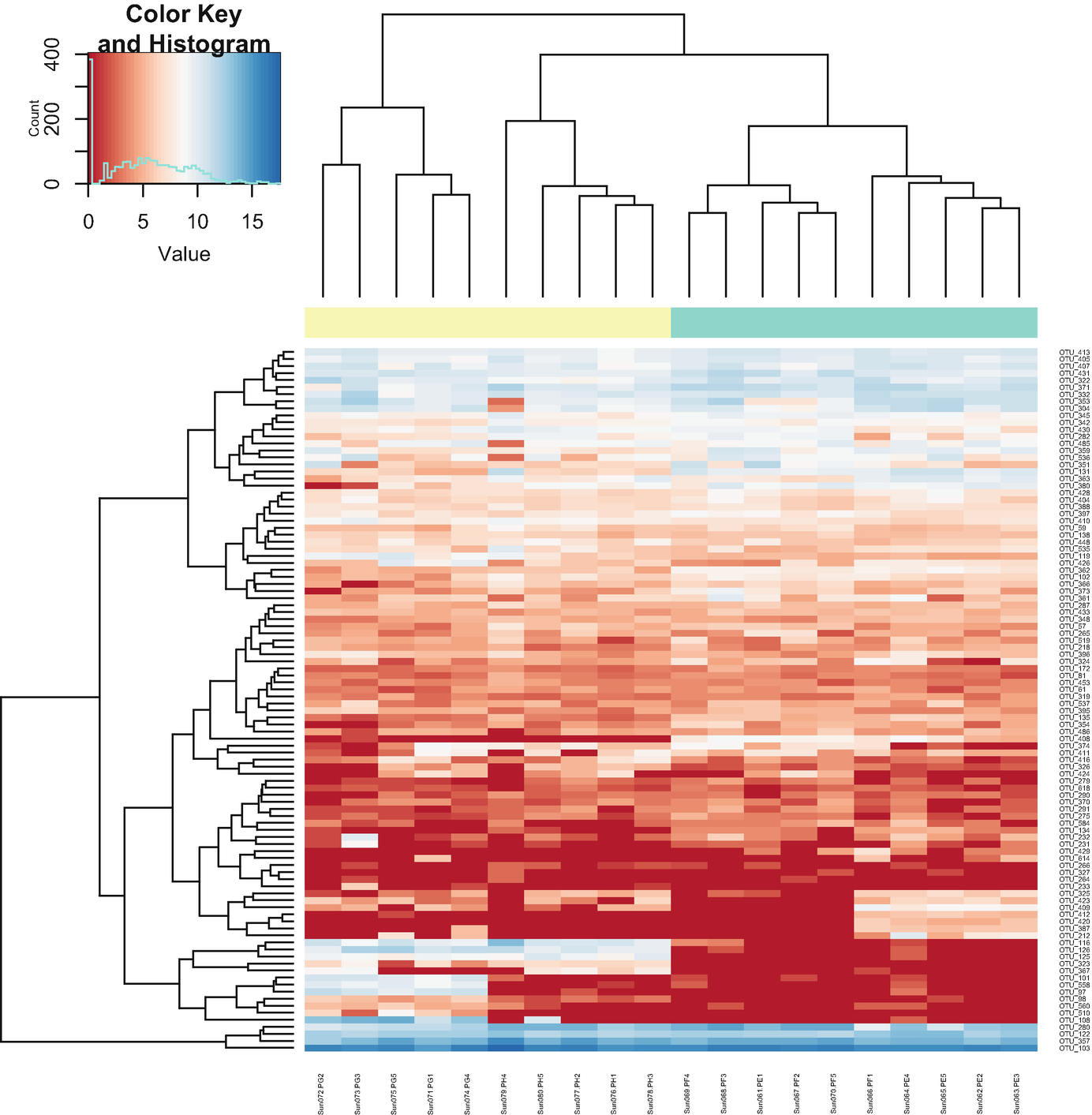
A heatmap and hierarchical cluster exhibit the abundance estimates. An inset graph of count versus value exposes the color key and histogram. The values are estimated between 0 and 15.

The above commands create a heatmap and hierarchical clustering of log₂ transformed counts for the 100 OTUs with the largest overall variance. Red values indicate counts close to zero. Row color labels indicate OTU taxonomic class; column color labels indicate genotype (yellow = KO, green = WT). Notice that the samples are obviously clustered by genotypes.

• Step 6b: plotCorr – heatmap of pairwise correlations (Fig. 12.2).

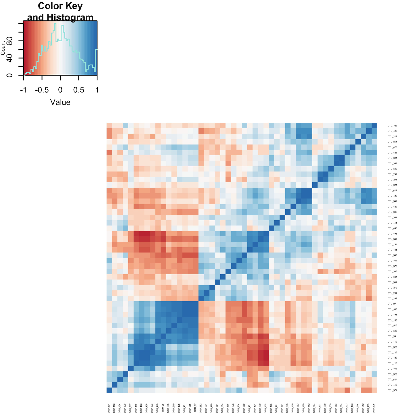
A heatmap exhibits the pairwise correlations. An inset graph of count versus value exposes the color key and histogram. The counts are estimated between 0 and 80.

• Step 6c: plotOrd – PCA/MDS components (Fig. 12.3).

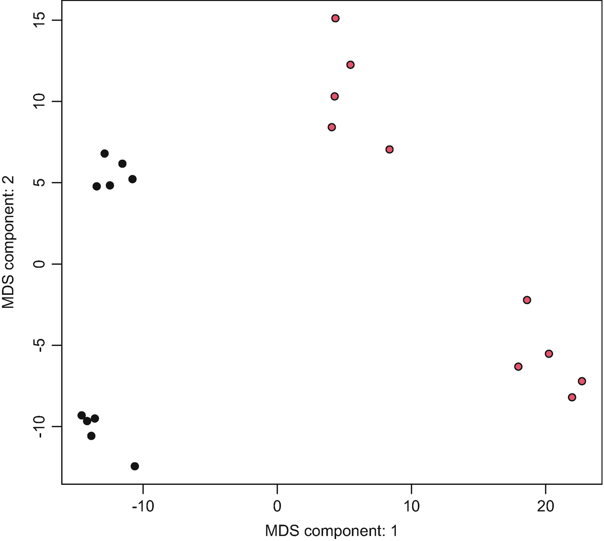
A graph of M D S component: 2 versus M D S component: 1 exhibits the C M D S plots. The plots were approximated between negative 10 to 20 along the x-axis and negative 10 to 15 along the y-axis.

We can also load the vegan package and set distfun = vegdist and use dist.method = ‘bray’ to generate the PCA using the Bray-Curtis dissimilarity method.

12.3 Some Additional Statistical Tests in metagenomeSeq

Below we will illustrate some useful tests in the metagenomeSeq package.

12.4 Illustrate Some Useful Functions in metagenomeSeq

To facilitate analysis using the metagenomeSeq package, we illustrate some useful functions.

12.5 Remarks on CSS Normalization, ZIG, and ZILN

CSS method divides raw counts into the cumulative sum of counts up to a percentile determined using a data-driven approach, which is an adaptive extension of the quantile normalization method (Bullard et al. 2010). CSS normalization may have the advantages, including the following: (1) CSS may have superior performance for weighted metrics, although it is arguable (Paulson et al. 2013, 2014; Costea et al. 2014; Weiss et al. 2017). (2) CSS is similar to log upper quartile (LUQ), but it is flexible than LUQ because it allows a dependent threshold to determine each sample’s quantile divisor (Weiss et al. 2017). (3) It was shown that CSS along with GMPR is overall more robust to sample-specific outlier OTUs than TSS and RNA-seq normalization methods (Chen et al. 2018). For CSS, it is crucial to ensure that chosen quantile is appropriate so that the normalization approach does not introduce normalization-related artifacts in the data, in which the normalization method assumes that all the count distributions of samples are roughly equivalent and independent of each other up to this quantile. However, the challenge is that the percentiles that CSS is based on could not be determined for microbiome datasets with high variable counts (Chen et al. 2018).

So far, most performances of metagenomeSeq have been evaluated based on ZIG; recently, one study demonstrated that ZILN mixture model successfully controls the FDR under 5% in all simulations, but suffers a severe loss of power (Lin and Peddada 2020a). Additional evaluations based on the ZILN are needed for providing further information on the metagenomeSeq methods.

12.6 Summary

In this chapter, we focused on introducing the metagenomeSeq methods including ZIG and ZILN mixture models as well as additional statistical tests and useful functions in metagenomeSeq. We first introduced TSS and CSS normalization methods. CSS is one critical component of the metagenomeSeq methods. We then described the ZIG and ZILN models. Next, we illustrated how to implement ZILN via the metagenomeSeq package. Currently ZILN or fitFeatureModel() function is recommended for use over ZIG functions or fitZig() function in the metagenomeSeq manual. Followed that, we illustrated some additional statistical tests that are available in metagenomeSeq: log-normal permutation test of abundance, presence-absence testing of the proportion/odds, discovery odds ratio testing of the proportion of observed counts, as well as performing feature correlations. To facilitate analysis of microbiome using the metagenomeSeq methods, we also illustrated some useful functions in metagenomeSeq to access the MRexperiment object, subset the MRexperiment object, filter the MRexperiment object or count matrix, merge the MRexperiment object, call the normalized counts using the cumNormMat() and MRcounts(), calculate the normalization factors using the calcNormFactors(), access the library sizes using the libSize(), save the normalized counts using the exportMat(), save the sample statistics using the exportStats(), find unique OTUs or features, and aggregate taxa and samples. Finally, we provided some remarks on CSS, ZIG, and ZILN.

In Chap. 13, we will introduce zero-inflated beta models for microbiome data.