Generalized linear mixed-effects models (GLMMs) and the generalized estimating equations (GEEs) are the two most appealing paradigms in a longitudinal setting. Thus, GEEs and GLMMs not only have been adopted for the analysis of longitudinal microbiome data at the beginning stage of microbiome research, but also have been used as a statistical foundation to build statistical models that specifically target longitudinal microbiome data in recent years. In Chap. 16, we investigated some general topics of GLMMs. Microbiome count data are often over-dispersed and zero-inflated, containing excess zeros than would be expected from the typical error distributions. In this chapter, we introduce GLMMs, with focusing on some newly developed GLMMs that take account for correlated observations with random effects while considering over-dispersion and zero-inflation. In Sect. 17.1, we review and discuss some general issues of GLMMs in microbiome research. Then, we introduce three GLMMs that can be used for modeling over-dispersed and zero-inflated longitudinal microbiome data. They are generalized linear mixed modeling (1) using glmmTMB package (Sect. 17.2); (2) using GLMMadaptive package (Sect. 17.3); and (3) fast zero-inflated negative binomial mixed modeling (FZINBMM) using the NBZIMM package (Sect. 17.4), which was specifically designed for analyzing longitudinal microbiome data. In Sect. 17.5, we provide some remarks on fitting GLMMs. Finally, we summarize this chapter in Sect. 17.6.
17.1 Generalized Linear Mixed Models (GLMMs) in Microbiome Research
In longitudinal study or repeated measurements, the observations on the same individual are often correlated, which is usually modeled with a random effect in generalized linear mixed models (GLMMs). Count data are typically modeled with GLMs and GLMMs using either Poisson or negative binomial distributions. However, microbiome count data are over-dispersed and sparse and often contain many zeros. Thus, Poisson model is not able to analyze microbiome count data due to its assumption of equality of the variance and the mean. The negative binomial model and its extensions are usually used to analyze the over-dispersed microbiome data. To model zero-inflated microbiome data, the zero-inflated or zero-hurdle models with the negative binomial distribution (a mixture of Poisson distributions with Gamma-distributed rates) can be applied. Xia et al. (2018a, b) introduced over-dispersed and zero-inflated modeling microbiome data.
In our 2018 book, we mainly adopted two widely used negative binomial (NB) models edgeR and DESeq2 in RNA-seq literature to model over-dispersed microbiome data as well as the widely-used pscl package to fit zero-inflated and zero-hurdle GLMs using maximum likelihood estimation (MLE) (Zeileis et al. 2008) along with various model comparisons.
A negative binomial (NB) model can model over-dispersion due to clustering and but cannot model over-dispersion, sparsity caused by zero-inflation, which could result in biased parameter estimates (Xia et al. 2018a; Xia 2020). We concluded that the zero-inflated and zero-hurdle GLMs with NB regression, i.e., zero-inflated negative binomial (ZINB) and zero-hurdle negative binomial (ZHNB) are the best fitted models to over-dispersed and zero-inflated microbiome data among the competing models including Poisson, NB, zero-inflated Poisson(ZIP), and zero-hurdle Poisson (ZHP) (Xia et al. 2018b).
However, pscl is not equipped with the component of random effects and thus is limited to cross-sectional data and cannot model longitudinal data or repeated measurements. Without modeling random effects and thereby ignoring correlation could lead the statistical inference to be anti-conservative (Bolker et al. 2009; Bolker 2015). Here, we introduce other two R packages glmmTMB and GLMMadaptive that can be used to model over-dispersed and zero-inflated longitudinal microbiome data. After the introduction of glmmTMB and GLMMadaptive, we will move on modeling microbiome data from GLMs, GLMMs, to zero-inflated generalized linear mixed models (ZIGLMMs). Before we move on to introducing the glmmTMB and GLMMadaptive packages, in this section, we review and introduce some specific issues in modeling microbiome data, including data transformation, challenges of model selection, and statistical hypothesis testing in microbiome data when using GLMMs.
17.1.1 Data Transformation Versus Using GLMMs
Log transformation usually only can remove or reduce skewness of the original data that follows a log-normal distribution or approximately so, which in some cases comes at the cost of actually making the distribution more skewed than the original data.
It is not generally true that the log transformation can reduce variability of data especially if the data includes outliers. In fact, whether or not log transformation can reduce variability depends on the magnitude of the mean of the observations — the larger the mean, the smaller the variability.
It is difficult to interpret model estimates from log transformed data because the results obtained from standard statistical tests on log-transformed data are often not relevant to the original, non-transformed data. In practice, the obtained model estimates from fitting the transformed data are usually required to translate back to the original scale through exponentiation to give a straightforward biological interpretation (Bland and Altman 1996). However, since no inverse function can map back exp(E(log X)) to the original scale in a meaningful fashion, it was advised that all interpretations should focus on the transformed scale once data are log-transformed (Feng et al. 2013).
Fundamentally, statistical hypothesis testing of equality of (arithmetic) means of two samples is different from testing equality of (geometric) means of two samples after log transformation of right-skewed data. These two hypothesis tests are equivalent if and only if the two samples have equivalent standard deviations.
The underlying assumption of the log transformation is that the transformed data have a distribution equal or close to the normal distribution (Feng et al. 2013). Since this assumption is often violated, therefore, log transformation with adding the shift parameter on the one hand cannot help reduce the variability and on the another hand could be quite problematic to test the equality of means of two samples when there are values close to zero in the samples. Actually even nonparametric models still need assumptions (e.g., homogeneity of variance across groups). Thus, the over-dispersed and zero-inflated count models are recommended (Xia et al. 2018a, b).
17.1.2 Model Selection in Microbiome Data
In general, nested models are compared using likelihood or score test, for example, to compare ZIP vs. ZINB (ZIP is nested within ZINB) and ZHP vs. ZHNB (ZHP nested within ZHNB), while non-nested models are evaluated using AIC and/or the Vuong test (Long 1997; Vuong 1989).
In statistical theory, AIC (Akaike 1973, 1998) and BIC (Schwarz 1978; Wit et al. 2012) have served as a common criterion (or the golden rules) for model selection since they were proposed (Aho et al. 2014).
In GLMMs, estimates of AIC have been developed based on certain exponential family distributions (Saefken et al. 2014). As we described in Chap. 16 (Sect. 16.5.3 of Information Criteria for Model Selection), AIC and BIC have several theoretical properties: consistency in selection, asymptotic efficiency, and minimax-rate optimality. For example, it was shown that AIC is asymptotically efficient for the nonparametric framework and is also minimax optimal (Barron et al. 1999) and BIC is consistent and asymptotically efficient for the parametric framework. However, AIC and BIC also have their own drawbacks. For example, AIC is inconsistent in a parametric framework (at least exist two correct candidate models), and hence AIC is not asymptotically efficient in such a framework. Actually it is difficult to evaluate analytically the properties of AIC for small samples, and thus its statistical optimality could not be demonstrated (Shibata 1976). BIC, on the other hand, is not minimax optimal and asymptotically efficient in a nonparametric framework (Shao 1997; Foster and George 1994). For the details on the good properties and drawbacks of AIC and BIC, the reader is referred to Ding et al. (2018a, b) for general references on these topics. In order to leverage the strengths of AIC and BIC and overcome their weaknesses, hybrid or adaptive approaches of AIC and BIC have been proposed such as in these cited references (Ing 2007; Yang 2007; Liu and Yang 2011; van Erven et al. 2012; Zhang and Yang 2015; Ding et al. 2018a).
Generally, AIC and BIC are sufficient to be used to choose better models. Various variants of AIC and BIC may not improve the decision too much. However, relying solely on AIC may misinterpret the importance of the variables in the set of candidate models; thus, combining AIC and BIC (BIC is more appropriate for heterogeneous data due to using more penalties) is recommended in modeling microbiome data in GLMMs.
- 1.
Over-dispersed and zero-inflated models are usually more appropriate than their nested (simple) models. Since generally it is obvious that NB models have advantages compared to their nested Poisson models, similarly, zero-inflated NB and zero-hurdle NB models have advantages than their nested zero-inflated Poisson and zero-hurdle Poisson models; thus, the information-theoretic approach is much more important than the null hypothesis testing approach.
- 2.
Most often the information-theoretic approach and the null hypothesis testing approach can provide consistent results for choosing the best models. Compared to ecology, model selection is relatively simple in microbiome study. Based on our experience, usually the test results from AIC, BIC, Vuong test, and LRT are consistent in microbiome data (Xia et al. 2018b). Considering them jointly should enable to choose a better model.
For the improvements of various variants of AIC and BIC, the readers can read the description of their properties and characteristics in Chap. 16 (Sect. 16.5.3).
17.1.3 Statistical Hypothesis Testing in Microbiome Data
First, the statistical methods that are appropriate for testing over-dispersion and zero-inflation are limited.
Second, testing the null hypothesis on the boundary poses more challenge on most statistical tests.
Third, choosing an appropriate method to calculate the degrees of freedom is difficult.
Wald t or F tests or AIC (AICc) needs to calculate the degrees of freedom (df), which is between 1 and the number of random-effect levels N − 1. Several approaches are available for calculating df and different software packages use different ones. But there is no consensus on which one is appropriate. For example, the simplest approach is the minimum number of df, which is contributed by random effects that affect the term being tested. SAS uses this approach as default (Littell et al. 2006). While the more complicated approach uses Satterthwaite and Kenward-Roger (KR) approximations of the degrees of freedom to adjust for the standard errors (Littell et al. 2006; Schaalje et al. 2001). KR (only available in SAS) was reviewed having overall best performance at least for LMMs (Schaalje et al. 2002; Bolker et al. 2009). Additionally, the residual df can be estimated by the sample size n minus the trace t (i.e., the sum of the diagonal elements) of the hat matrix (Burnham 1998; Spiegelhalter et al. 2002). Due to the complexity, the calculating degrees of freedom and boundary effects have been reviewed as the two particular challenges to perform statistical testing the results of GLMMs (Bolker et al. 2009).
17.2 Generalized Linear Mixed Modeling Using the glmmTMB Package
In this section, we introduce the glmmTMB package and illustrate its use with microbiome data.
17.2.1 Introduction to glmmTMB
The R package glmmTMB (Brooks et al. 2017) was developed to estimate GLMs and GLMMs and to extend the GLMMs by including zero-inflated and hurdle GLMMs using ML. Thus, glmmTMB can handle a various range of statistical distributions including Gaussian, Poisson, binomial, negative binomial, and beta. Because glmmTMB extended GLMMs, it can not only model zero-inflation, heteroscedasticity, and autocorrelation but also handle various types of within-subject correlation structures.
The glmmTMB package has wrapped all these capabilities of estimates in GLMs, GLMMs, and their extensions including zero-inflated and hurdle GLMMs using ML. Currently glmmTMB focuses on zero-inflated counts although this package can be used to fit continuous distributions too (Brooks et al. 2017).
The zero-inflated (more broadly zero-altered) models wrapped in glmmTMB was developed under the framework of GLMs and GLMMs, which allow us to model count data using a mixture of a Poisson, NB. Especially glmmTMB uses the Conway-Maxwell-Poisson distribution (Huang 2017), which consists of both mean and dispersion parameters. It is a generalized version of the Poisson distribution with the Bernoulli and geometric distributions as special cases (Sellers and Shmueli 2010). Depending on the dispersion, Conway-Maxwell-Poisson distribution can have either longer or shorter upper tail than that of the Poisson (Sellers and Shmueli 2010). Thus, it can model either over- or under-dispersed count data (Shmueli et al. 2005; Lynch et al. 2014; Barriga and Louzada 2014; Brooks et al. 2017). Conway-Maxwell-Poisson distribution can flexibly model dispersion and skewness through the Sichel and Delaporte distributions (Stasinopoulos et al. 2017).
The glmmTMB package uses the interface and formula syntax of the lme4 package (Bates et al. 2015) and performs estimation via the TMB (Template Model Builder) package (Kristensen et al. 2016). Like lme4, glmmTMB uses MLE and the Laplace approximation to integrate over random effects. Currently the restricted maximum likelihood (REML) is not available in glmmTMB, and the random effects are not integrated using the Gauss-Hermite quadrature, although they are available in lme4 (Brooks et al. 2017). However, a fundamental difference underlying implementation between glmmTMB and lme4 is that glmmTMB uses TMB to take the advantage of fast estimating non-Gaussian models and provides more flexibility to fit the classes of distributions that it can fit (Brooks et al. 2017).
A glmmTMB model consists of four main components: (1) a conditional model formula, (2) a distribution for the conditional model, (3) a dispersion model formula, and (4) a zero-inflation model formula. Both fixed and random effects models can be specified in the conditional and zero-inflated components of the model. For the dispersion parameter, only the fixed effects models can be specified.
17.2.1.1 Conditional Model Formula
counts vary by taxon and vary randomly by subject.

The above model formulation in (17.1) allows the conditional mean to depend on whether or not a subject was from covariate 1 (group variable, e.g., treatment vs. control) and to vary randomly by subject. It also allows the number of structural (i.e., extra) zeros to depend on covariate 1 (group variable). Additionally, it allows the dispersion parameter to depend on covariate 2 (e.g., time).
17.2.1.2 Distribution for the Conditional Model
We can specify the distribution of the mean of the conditional model via the family argument. For the count data, the family of the distribution includes Poisson (family = poisson), negative binomial (family = nbinom1 or family = nbinom2), and Conway-Maxwell-Poisson to fit over- and under-dispersed data (family = compois). By default, the link function of Poisson, Conway-Maxwell-Poisson, and negative binomial distributions is log. We can specify other links using the family argument such as family = poisson(link = “identity”).
glmmTMB provides two parameterizations of the negative binomial. They are different in the dependence of the variance (σ2) on the mean (μ). The argument family = nbinom1 is used to indicate that the variance increases linearly with the mean, i.e., σ2 = μ(1 + α), with α > 0; while the argument family = nbinom2 is used to indicate that the variance increases quadratically with the mean, i.e., σ2 = μ(1 +μ/𝜃), with θ >0 (Hardin et al. 2007). The variance of the Conway-Maxwell-Poisson distribution does not have a closed form equation (Huang 2017).
17.2.1.3 Dispersion Model Formula
In glmmTMB, the dispersion parameter can be specified as either identical dispersion or covariate-dependent dispersion. For example, the default dispersion model (dispformula = ~1) treats the dispersion parameter (e.g., α or θ in the NB model) as identical for each observation; while the dispersion parameter can also be treated as varying with fixed effects, in which the dispersion model uses a log link. We can also use the dispersion model to account for heteroskedasticity. For example, to account for more variation (relative to the mean) of the response to a predictor variable, we can specify the one-sided formula dispformula = ~ this predictor variable in a NB distribution. Although when the conditional and dispersion models include the same variables, the mean-variance relationship can be manipulated; however, a potential non-convergence issue could happen (Brooks et al. 2017). To see the description of the dispersion parameter for each distribution, type?sigma.glmmTMB in R or RStudio.
17.2.1.4 Zero-Inflation Model Formula
The overall distribution of zero-inflated generalized models is a mixture of the conditional model and zero-inflation model (Lambert 1992). The zero-inflation model describes the probability of observing an extra (i.e., structural) zero that is not generated by the conditional model. Zero-inflation model creates an extra point mass of zeros in the response distribution, where the zero-inflation probability is bounded between zero and one by using a logit link.
To assume that the probability of producing a structural zero for all observations is equal, we can specify an intercept model as ziformula = ~1 to account for the structural zero. To model the structural zero of the response due to a specific predictor variable, we can specify ziformula = ~ this predictor variable in the zero-inflation model. glmmTMB also allows to include random effects in both conditional and zero-inflation models, but not allowing to specify a term of random effects in the dispersion model.
17.2.2 Implement GLMMs via glmmTMB
This dataset was used in previous chapters. Here we continue to use this dataset to illustrate glmmTMB. The 16S rRNA microbiome data were measured at pretreatment and posttreatment times for 10 samples at each time. We are interested in the differences between the genotype factors or groups. We use the example data to illustrate how to fit and compare GLMMs, zero-inflated GLMMs, and hurdle GLMMs using glmmTMB and how to extract results from a model.
Here, we illustrate how to perform model selection to select the models that are better fitted to this abundance data in detecting the genotype differences. The compared models include Poisson, Conway-Maxwell-Poisson, negative binomial, zero-inflated, and zero-hurdle models. We use the species “D_6__Ruminiclostridium.sp.KB18” for this illusttration.
To run the glmmTMB() function to perform GLMMs, we first need to install the glmmTMB package, which is available from the Comprehensive R Archive Network (CRAN) (current version 1.1.2.3, February 2022) and from GitHub (development versions). We can install glmmTMB via CRAN using the command install.packages(“glmmTMB”) or via GitHub using devtools (Wickham and Chang 2017): devtools::install_github(“glmmTMB/glmmTMB/glmmTMB”).
Step 1: Load taxa abundance data and meta data.
Step 2: Check taxa and meta data.
Step 3: Create analysis dataset including outcomes and covariates.
Step 4: Explore the distributions of the outcomes (taxa).
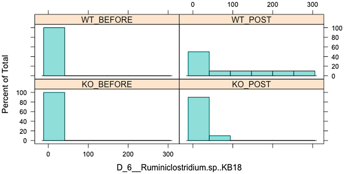
A bar graph of percent of total versus D underscore 6 underscore Ruminiclostridium dot s p, K B 18 has 4 parts, W T before, W T post, K O before, and K O post. The graph follows a decreasing trend.
Histogram of Ruminiclostridium.sp.KB18 over before and posttreatment in wild-type (WT) and knockout (KO) groups
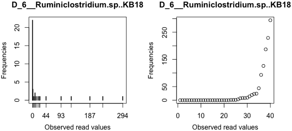
A graph and a scatterplot of D underscore 6 underscore Ruminiclostridium dot s p, K B 18 plots frequencies versus observed read values. The graph displays a decreasing trend and the scatterplot has an increasing trend.
Distribution of Ruminiclostridium.sp.KB18
Step 5: Run the glmmTMB() function to implement glmmTMB.
For each outcome taxonomy variable (here, D_6__Ruminiclostridium.sp.KB18), we fit fixed effects of two main factors Group, Time, and their interaction term. For random effects, we specify that taxonomy counts vary randomly by mouse.
(family = nbinom1)
(family = nbinom2)
(family = nbinom1 and disp = ~Time)
(family = nbinom2 and disp = ~Time)
ZIP(family= poisson and zi = ~ Group)
When a model is overparameterized, then the data does not contain enough information to estimate the parameters reliably.
When a random-effect variance is estimated to be zero, or random-effect terms are estimated to be perfectly correlated (“singular fit”).
When zero-inflation is estimated to be near zero (a strongly negative zero-inflation parameter).
When dispersion is estimated to be near zero.
When complete separation occurs in a binomial model: some categories in the model contain proportions that are either all 0 or all 1.
Commonly these problems are typically caused by trying to estimate parameters for which the data do not contain information, such as a zero-inflated and over-dispersed model is specified for the data that does not have zero-inflation and/or over-dispersion, or a random effect is assumed for varying not necessary predictors. The general model convergence issues are discussed in vignette (“troubleshooting”). The readers are referred to this vignette to obtain advice for troubleshooting convergence issues that have been developed (“troubleshooting”, package = “glmmTMB”). For the detailed estimation challenges in GLMMs, The readers are referred to Sect. 17.1.3.
ZICMP(family = compois and zi = ~ Group as well as zi = ~ Group*Time)
ZINB(family = nbinom1 and zi = ~ Group*Time)
ZINB(family = nbinom2 and zi = ~ Group)
Since zinb2a does not converge, we specify zi = ~ Group in below zinb2 instead.
ZHP(family = truncated_poisson and zi = ~ Group*Time)
ZHNB (family = truncated_nbinom1/truncated_nbinom2 and zi = ~ Group*Time)
Step 6: Perform model comparison and model selection using AIC and BIC.
Model comparison using AIC and BIC and offset.
Model comparison using AIC and BIC but without offset.
Both AICtab () and BICtab()functions report the log-likelihood of the unconverged models as NA at the end of the AIC and BIC tables.
AIC and BIC values in compared models from glmmTMB
Model | No offset | Using offset | ||
|---|---|---|---|---|
AIC | BIC | AIC | BIC | |
zhnb2 | 201.3 | 218.2 | NA | NA |
zhp | 202.1 | 217.3 | 203.2 | 218.4 |
zicmp0 | 202.5 | 219.4 | 204.0 | 220.9 |
zinb2 | 203.1 | 216.6 | 204.3 | 217.9 |
zicmp | 203.1 | 216.6 | 204.7 | 218.2 |
zhnb1 | 203.6 | 220.5 | NA | NA |
zinb1 | 205.4 | 222.3 | NA | NA |
nb2 | 220.6 | 230.8 | 220.7 | 230.9 |
nbdisp2 | 222.5 | 234.4 | 222.6 | 234.5 |
nbdisp1 | 223.9 | 235.7 | 224.2 | 236.0 |
nb1 | 224.5 | 234.6 | 225.1 | 235.2 |
zip | 229.9 | 241.7 | 205.7 | 217.5 |
cmpoi | 231.0 | 241.1 | 231.4 | 241.5 |
poi | 295.9 | 304.3 | 298.3 | 306.7 |
zip0 | NA | NA | 205.6 | 220.8 |
zinb1a | NA | NA | NA | NA |
From Table 17.1, we can see using offset does not improve model fit for this specific outcome variable: either there are more non-converged models using offset or more models have slightly worse model fits. Using offsets only zero-inflated models have better model fits than those without using offsets, but some warning messages are generated, so the model evaluation is suspicious.
Step 7: Perform residual diagnostics for GLMMs using DHARMa.
We can evaluate the goodness-of-fit of fitted GLMMs using the procedures described in the DHARMa package (version 0.4.5, 2022-01-16). The R package DHARMa (or strictly speaking, DHARM) (Hartig 2022) stands for “Diagnostics for HierArchical Regression Models.” The name DHARMa is used to avoid confusion with the term Darm which in German means intestines and also taking the meaning of DHARMa in Hinduism which signifies behaviors should be in accord with rta, the order that makes life and universe possible, including duties, rights, laws, conduct, virtues, and “right way of living.” The meaning of DHARMa in Hinduism is purposed to play for this package, i.e., to test whether fitted model is in harmony with the data tested.
DHARMa uses a simulation-based approach to create readily interpretable scaled (quantile) residuals for fitted (generalized) linear mixed models. Currently the linear and generalized linear (mixed) models supported by DHARMa are from “lme4” (classes “lmerMod,” “glmerMod”), “glmmTMB,” “GLMMadaptive” and “spam,” generalized additive models (“gam” from “mgcv”), “glm” (including “negbin” from “MASS,” but not quasi-distributions), and “lm” model classes.
DHARMa standardizes the resulting residuals to values between 0 and 1. Thus, the residuals can be intuitively interpreted as residuals from a linear regression. There are two basic steps behind the residual method: (1) Simulate new response data from the fitted model for each observation. (2) For each observation, calculate the empirical cumulative density function for the simulated observations, which describes the possible values and their probability given the observed predictors and assuming the fitted model is correct. The residual generated this way represents the value of the empirical density function at the value of the observed data. Thus, a residual of 0 means that all simulated values are larger than the observed value, and a residual of 0.5 means that half of the simulated values are larger than the observed value (Dunn and Smyth 1996; Gelman and Hill 2006).
The package provides a number of plot and test functions for diagnosing typical model misspecification problems, including over−/under-dispersion and zero-inflation.
Step 7a: Simulate and plot the scaled residuals from the fitted model using the functions simulateResiduals() and plot.DHARMa().
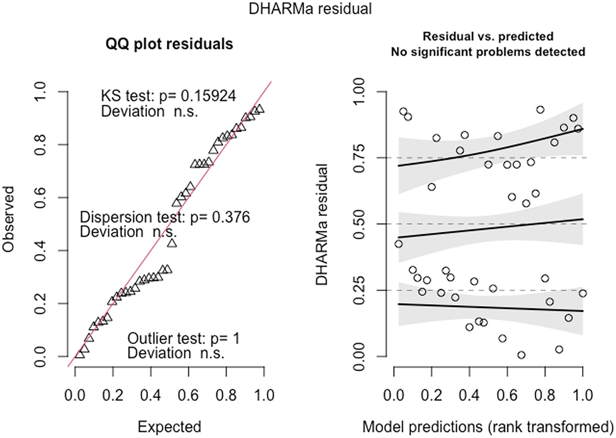
2 scatterplots. 1. A scatterplot of Q Q plot residuals plots observed versus expected. It exhibits an increasing trend. 2. A scatterplot of D H A R M a residual versus model predictions has an increasing trend.
QQ-plot residuals (left panel) and the scatterplot of the residuals against the predicted (fitted) values plot (right panel) in fitted Poisson model by the glmmTMB package
The QQ-plot of the observed versus expected residuals is created by the plotQQunif () function to detect overall deviations from the expected distribution. The scaled residuals have a uniform distribution in the interval (0,1) for a well-specified model. The P-value reported in the plot is obtained from the Kolmogorov-Smirnov test for testing uniformity. By default, the three generated tests are KS test (for correct distribution), dispersion test (for detecting dispersion), and outlier test (for detecting outliers). The plot generated by the plotResiduals () by default is the residuals against the predicted values, but the plot of the residuals against specific predictors is highly recommended. To visualize the effects in detecting deviations from uniformity in y-direction, the plot function also calculates a quantile regression to compare the empirical 0.25, 0.5, and 0.75 quantile lines across the plots in y-direction. These lines should be straight, horizontal, and at y-values of the theoretical 0.25, 0.5, and 0.75 quantiles.
Step 7b: Perform goodness-of-fit tests on the simulated scaled residuals.
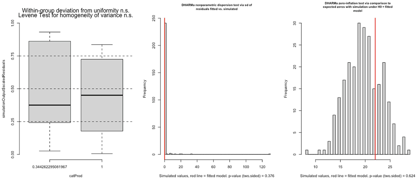
3 graphs. A. A boxplot of simulation outputs scaled residuals versus cat Pred has 2 boxes. B and C. 2 histograms of frequency versus simulated value with p-value equals 0.376 and p equals 0.624, respectively.
Levene test for homogeneity of variance (left panel), nonparametric dispersion test (middle panel), and zero-inflation test (right panel) for fitted Poisson model by the glmmTMB package
In this case, both dispersion and zero-inflation tests are not statistically significant.
In DHARMa, several overdispersion tests are available for comparing the dispersion of simulated residuals to the observed residuals. The syntax is given:
The default type is DHARMa, which is a non-parametric test to compare the variance of the simulated residuals to the observed residuals. Alternatively, it is PearsonChisq, which implements the Pearson-χ2 test. While if residual simulations are done via refit, DHARMa will compare the Pearson residuals of the re-fitted simulations to the original Pearson residuals. This is essentially a nonparametric test. The author of the DHARMa package showed that the default test is fast, nearly unbiased for testing both under and over-dispersion, as well as reliably powerful.
One important resource of over-dispersion is zero-inflation. In DHARMa, zero-inflation can be formally tested using the function testZeroInflation(), such as here testZeroInflation(SimulatedOutput_poi), to compare the distribution of expected zeros in the data against the observed zeros.
2 scatterplots. 1. A scatterplot of Q Q plot residuals plots observed versus expected. It depicts an increasing trend. 2. A scatterplot of D H A R M a residual versus model predictions. It exhibits a decreasing trend.
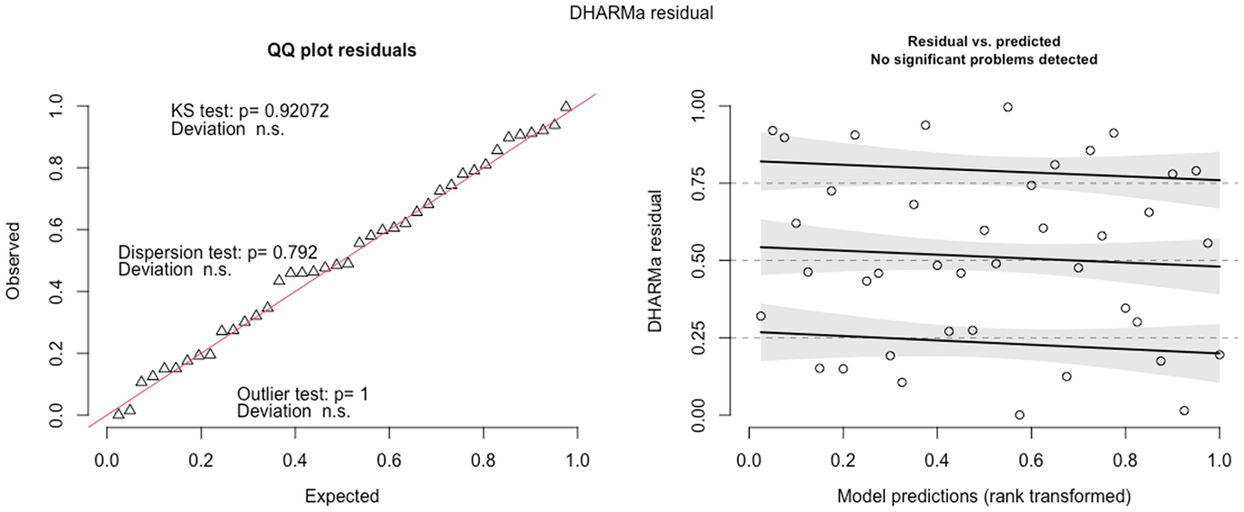
QQ-plot residuals (left panel) and Residuals vs. predicted values plot (right panel) in fitted zinb2 model by the glmmTMB package
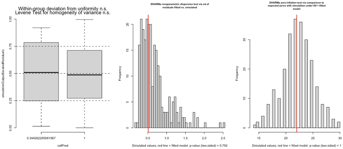
3 graphs. A. A box plot of simulation outputs scaled residuals versus cat Pred plots 2 boxes. B and C. 2 histograms of frequency versus simulated value with p-value equals 0.792 and p equals 1, respectively.
Levene test for homogeneity of variance (left panel), nonparametric dispersion test (middle panel), and zero-inflation test (right panel) for fitted zinb2 model by the glmmTMB package
Step 8: Summarize the modeling results and extract the outputs of selected models.
Modeling results from the models that use offset via glmmTMB
Model | Conditional model | ||||
|---|---|---|---|---|---|
Interaction term | Estimate | Std. Error | z value | P-value | |
poi | Group:TimePost | −4.939 | 0.606 | −8.15 | 3.6e-16 |
cmpoi | Group:TimePost | −4.347 | 1.032 | −4.21 | 2.6e-05 |
nb1 | Group:TimePost | −2.44 | 1.20 | −2.03 | 0.0425 |
nb2 | Group:TimePost | −4.905 | 1.512 | −3.24 | 0.0012 |
nbdisp1 | Group:TimePost | −1.669 | 1.107 | −1.51 | 0.13 |
nbdisp2 | Group:TimePost | −4.903 | 1.542 | −3.18 | 0.0015 |
zip0 | Group:TimePost | −6.879 | 0.645 | −10.67 | < 2e-16 |
zip | Group:TimePost | −6.291 | 0.732 | −8.59 | <2e-16 |
zicmp | Group:TimePost | −5.944 | 0.975 | −6.10 | 1.1e-09 |
zicmp0 | Group:TimePost | −6.423 | 0.909 | −7.07 | 1.6e-12 |
zinb1 | Group:TimePost | −5.827 | 0.939 | −6.21 | 5.4e-10 |
zinb2 | Group:TimePost | −5.936 | 0.858 | −6.92 | 4.6e-12 |
zhp | Group:TimePost | −24.8 | 11825.8 | 0 | 1 |
The following commands implement ZHP(family = truncated_poisson) and summarize the modeling results.
Modeling results from the models that do not use offset via glmmTMB
Model | Conditional model | ||||
|---|---|---|---|---|---|
Interaction term | Estimate | Std. Error | z value | P-value | |
poi | Group:TimePost | −4.678 | 0.606 | - 7.72 | 1.2e-14 |
cmpoi | Group:TimePost | −4.135 | 1.026 | −4.03 | 5.5e-05 |
nb1 | Group:TimePost | −2.230 | 1.130 | −1.97 | 0.04847 |
nb2 | Group:TimePost | −4.68 | 1.51 | - 3.10 | 0.0019 |
nbdisp1 | Group:TimePost | −1.478 | 1.114 | −1.33 | 0.18 |
nbdisp2 | Group:TimePost | −4.68 | 1.54 | −3.04 | 0.0024 |
zip | Group:TimePost | −6.037 | 0.627 | −9.63 | <2e-16 |
zicmp | Group:TimePost | −5.732 | 0.948 | −6.05 | 1.5e-09 |
zicmp0 | Group:TimePost | −6.271 | 0.857 | −7.32 | 2.5e-13 |
zinb1 | Group:TimePost | −6.247 | 0.937 | −6.67 | 2.6e-11 |
zinb2 | Group:TimePost | −5.711 | 0.840 | −6.80 | 1.1e-11 |
zhp | Group:TimePost | −23.9 | 8656.4 | 0 | 1 |
zhnb1 | Group:TimePost | −23.9 | 10093.7 | 0 | 1 |
zhnb2 | Group:TimePost | −23.8 | 8597.3 | 0 | 1 |
Group by TimePost interaction in conditional model is not statistically significant identified by truncated nbinom2 model.
Group by TimePost interaction in conditional model is statistically significant identified by zero-inflated nbinom2 model.
17.2.3 Remarks on glmmTMB
Various models including GLMs, GLMMs, zero-inflated GLMMs, and hurdle models can be quickly fitted in a single package.
The information criteria provided in the modeling results facilitates the model comparisons and model selection via using likelihood-based methods to compare the model fitting of the estimated models.
At least one simulation study in microbiome literature (Xinyan Zhang and Yi 2020b) confirmed that glmmTMB controlled the false-positive rates close to the significance level over different sample sizes, while remaining reasonable empirical power.
Estimating Conway-Maxwell-Poisson distribution is time expensive when the model is over-parameterized.
Convergence is an issue when the model is over specified with more than necessary predictors.
Based on AIC and BIC and conditional model in detecting significant interesting variables, we recommend using zinb (zinb1 and zinb2) and zicmp rather than zhp and zhnb (zhnb1 and zhnb2). They are all robust in modeling estimations and sensitive to identify significant interesting variables. The concept adjustment for using zero-hurdle and zero-inflated models, the readers are referred to Xia et al. (2018b).
The benefit of using offset has not been approved in microbiome research, and like the practice of sequencing depth rarefaction (rarefying sequencing to same depth), which is adopted from macro-ecology, the argument of using offset has not been solidly validated and is difficult to validate. In this study, we compared same GLMMs using and without using offset and found that the goodness-of-fit not necessarily improved by using offset based on AIC and BIC. Actually several advanced/completed GLMMs had model convergence problems. The non-improvement of using offset may be due to two reasons: (1) For univariate approach (using one taxon per time as the response variable), it is not appropriate or not necessary to adjust for sample total reads. (2) For advanced/completed GLMMs, it is a burden to add additional parameter to estimate.
17.3 Generalized Linear Mixed Modeling Using the GLMMadaptive Package
In this section, we introduce another R package GLMMadaptive and illustrate its use with microbiome data.
17.3.1 Introduction to GLMMadaptive
GLMMadaptive was developed by Dimitris Rizopoulos (2022a) to fit GLMMs for a single grouping factor under maximum likelihood approximating the integrals over the random effects. Unlike the lme4 and glmmTMB packages, this package uses an adaptive Gauss-Hermite quadrature (AGQ) rule (Pinheiro and Bates 1995). GLMMadaptive provides functions for fitting and post-processing mixed effects models for grouped/repeated measurements/clustered outcomes for which the integral over the random effects in the definition of the marginal likelihood cannot be solved analytically. This package fits mixed effects models for grouped/repeated measurements data which have a non-normal distribution, while allowing for multiple correlated random effects.
In GLMMadaptive, the AGQ rule is efficiently implemented to allow for specifying multiple correlated random effects terms for the grouping factor including random intercepts, random linear, and random quadratic slopes. It also offers several utility functions for extracting useful information from the fitted mixed effects models. Additionally, GLMMadaptive provides a hybrid optimization procedure: starting with implementing an EM algorithm, treating the random effects as “missing data,” and then performing a direct optimization procedure with a quasi-Newton algorithm.
17.3.2 Implement GLMMs via GLMMadaptive
mixed_model(fixed = y ~ x1 + x2, random = ~1 | g, data = df, family = zi.negative.binomial()).
fixed is a formula that is used for specifying the fixed effects including the response (outcome) variable.
random is a formula that is used for specifying the random effects.
family is a family object that is used for specifying the type of the repeatedly measured response variable (e.g., binomial() or poisson()).
data is a data frame containing the variables required in fixed and random.
In the mixed effects model, y denotes a grouped/clustered outcome, x1 and x2 denote the covariates, and g denotes the grouping factor. The above example syntax of mixed effects model specifies y as outcome and x1 and x2 as fixed effects and random intercepts. The mixed effects model is fitted by zero-inflated negative binomial model. If we also want to specify both intercepts and x1 as the random effects, then update the random = ~x1 | g (e.g., ~ time | id) in the call to mixed_model()function.
Family objects and models that can be fitted in GLMMadaptive
Family object | Model to fit |
|---|---|
negative.binomial() | Negative binomial |
zi.poisson() | Zero-inflated Poisson |
zi.negative.binomial() | Zero-inflated negative binomial |
hurdle.poisson() | Hurdle Poisson |
hurdle.negative.binomial() | Hurdle negative binomial |
hurdle.lognormal() | Two-part/hurdle mixed models for semi-continuous normal data |
censored.normal() | Mixed models for censored normal data |
cr_setup() and cr_marg_probs() | Continuation ratio mixed models for ordinal data |
beta.fam() | Beta |
hurdle.beta.fam() | Hurdle beta |
Gamma() or Gamma.fam() | Gamma mixed effects models |
censored.normal() | Linear mixed effects models with right and left censored data |
For the repeated measurements response variable, we may specify our own log-density function and use the internal algorithms for the optimization. The marginalized coefficients can be calculated via the marginal_coefs () using the approach of Hedeker et al. (2018) to calculate marginal coefficients from mixed models with nonlinear link functions. The GLMMadaptive package also provides predictions and their confidence intervals for constructing effects plots via the effectPlotData ().
Here, we first use the same example data in Example 17.1 to illustrate how to fit negative binomial, zero-inflated Poisson, zero-inflated negative binomial, hurdle Poisson, and hurdle negative binomial models using the GLMMadaptive package. We then illustrate how to perform model comparison and model selection to choose the best models. As we described in Example 17.1, the species “D_6__Ruminiclostridium.sp.KB18” has 30%, 50%, and 70% of zeros in genotype and wild-type (WT) groups before and posttreatments. We use this species to illustrate implmenting GLMMs using GLMMadaptive through the following six steps.
Step 1: Install package and load data.
To install the GLMMadaptive package (version 0.8-5, 2022-02-07), type the following commands in R or RStudio.
The development version of the GLMMadaptive package and its vignettes are available from GitHub, which can be installed using the devtools package:
Step 2: Create analysis dataset including outcomes and covariates.
Step 3: Fit candidated mixed models.
Step 4: Perform model comparisons and model selection.
Step 5: Evaluate goodness of fit using simulated residuals via the DHARMa package.
AIC and BIC values in compared models from GLMMadaptive
Model | AIC | BIC |
|---|---|---|
Zhp | 201.1 | 209.1 |
Zip | 203.7 | 214.7 |
Zinb | 205.8 | 217.7 |
Nb | 224.6 | 232.6 |
Zhnb | 226.2 | 235.2 |
Poi | 231.4 | 238.4 |
object is an object inheriting from class MixMod.
y is the observed response vector.
nsim is used to specify an integer number of simulated datasets(defaults is 1000).
type is what type of fitted values and data to simulate; it is used for including the random effects or setting them to zero.
integerResponse is a logical argument; it sets to TRUE for discrete grouped/cluster outcome data. Based on the chosen family for fitting the model, the integerResponse is automatically determined by this function. But for user-specified family objects, this argument needs to be defined by the user. Here, we evaluate the goodness-of-fit of the chosen family, so the integerResponse argument is automatically determined.
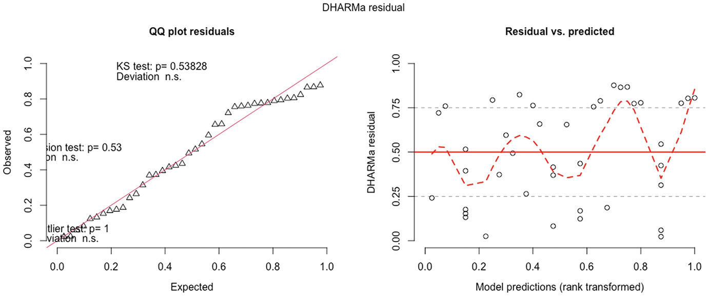
The following commands call the function resids_plot() and via the package DHARMa to generate two residual plots: QQ plot residuals on the left panel and residuals vs. predicted values (ranks transformed) on the right panel.
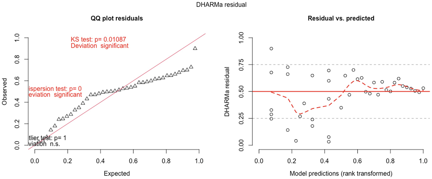
2 scatterplots. 1. A scatterplot of Q Q plot residuals plots observed versus expected. It exhibits an increasing trend. 2. A scatterplot of D H A R M a residual versus model predictions. It displays a fluctuating trend.
QQ-plot residuals (left panel) and residuals vs. predicted values plot(right panel) in fitted Poisson model by the GLMMadaptive package
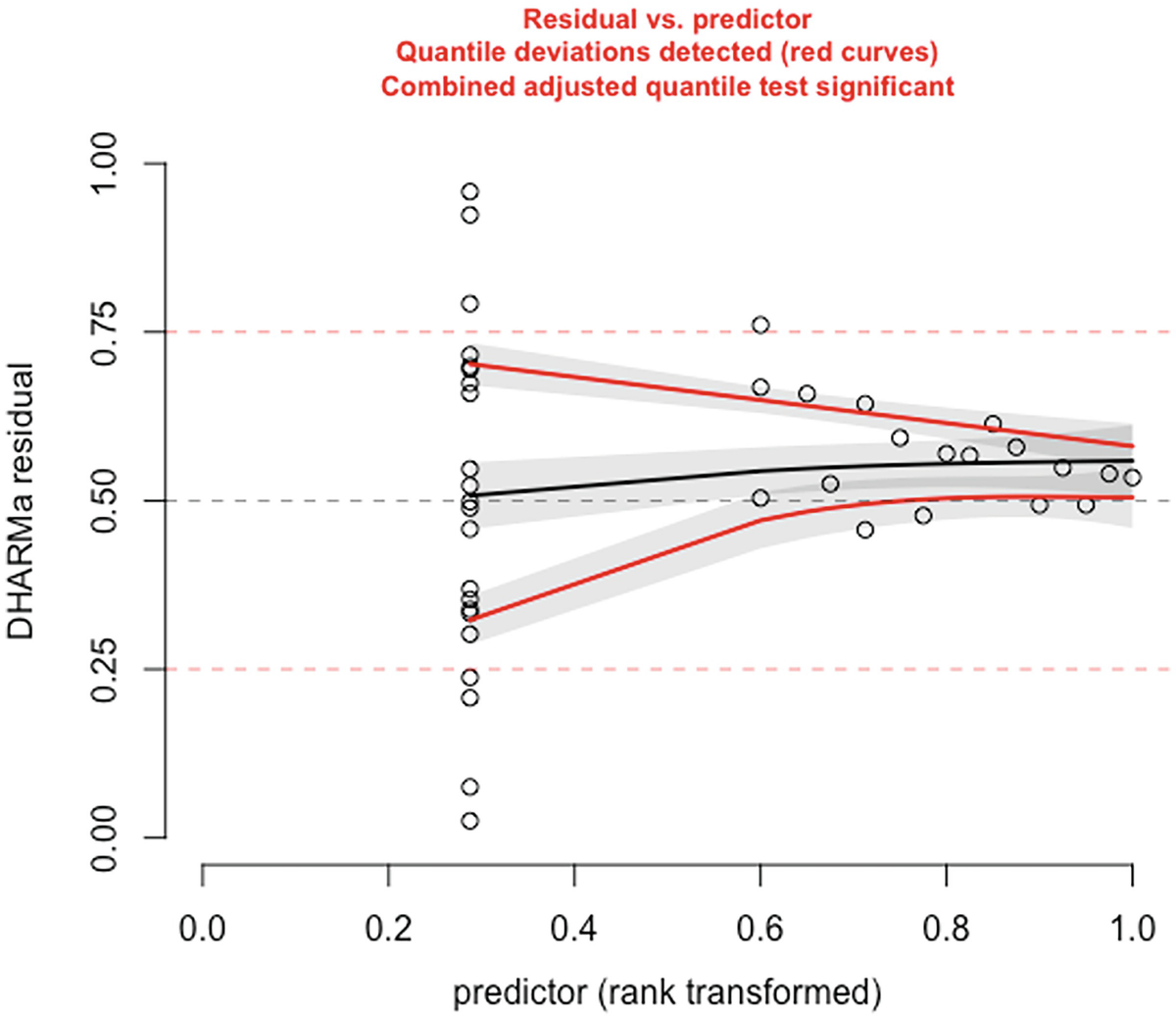
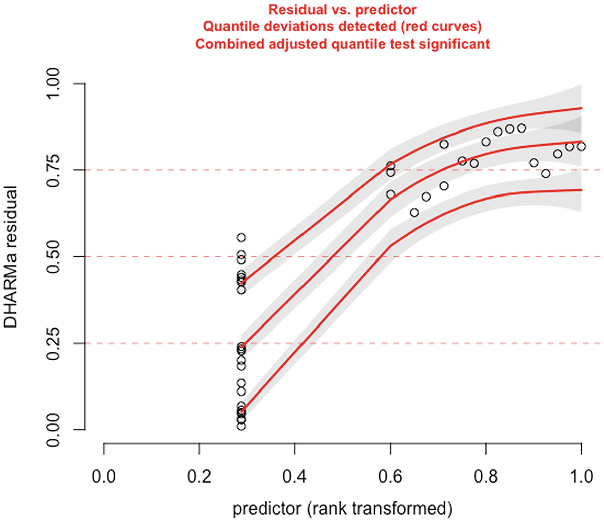
A scatterplot of D H A R M a residual versus predictor, rank transformed. It displays a decreasing red curve, an increasing black curve, and an increasing red curve. The red curves are plotted for detected quantile deviations.
The significance of the deviation of the empirical quantiles to the expected quantiles in fitted Poisson model is tested and visualized with the testQuantiles () function
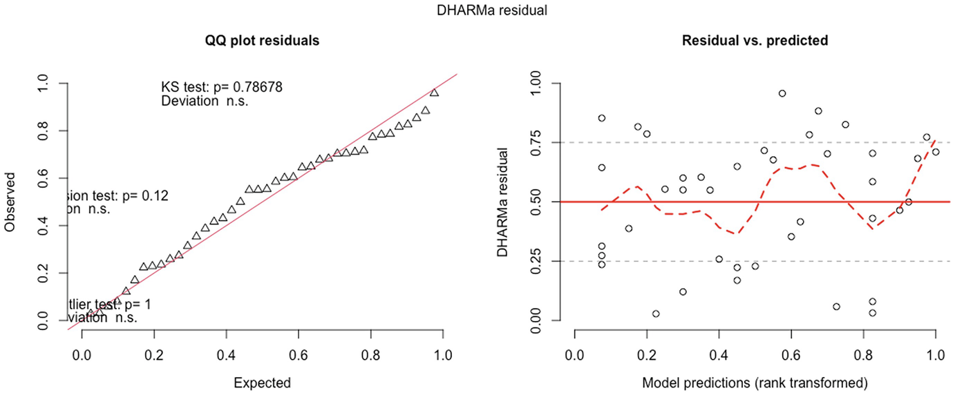
2 scatterplots. 1. A scatterplot of Q Q plot residuals plots observed versus expected. It has an increasing trend. 2. A scatterplot of D H A R M a residual versus model predictions has a fluctuating trend.
QQ-plot residuals (left panel) and residuals vs. predicted values plot (right panel) in fitted zero-truncated Poisson model by the GLMMadaptive package
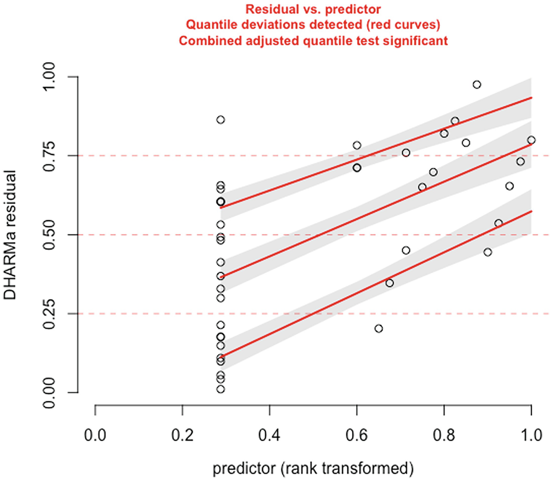
A scatterplot of D H A R M a residual versus predictor rank transformed. It exhibits an increasing trend with 3 increasing red curves for detected quantile deviations.
The significance of the deviation of the empirical quantiles to the expected quantiles in fitted zero-truncated Poisson model is tested and visualized with the testQuantiles () function
> # Figure 17.9
> resids_plot(zhp, ds$D_6__Ruminiclostridium.sp..KB18)
QQ-plot showed that the zero-truncated Poisson model has improved the model fit compared to the Poisson model. It seems to be acceptable. But based on the testing of the significance of the deviation of the empirical quantiles to the expected quantiles, the zero-truncated Poisson is still not well fitted.
2 scatterplots. 1. A scatterplot of Q Q plot residuals plots observed versus expected. It depicts an increasing trend. 2. A scatterplot of D H A R M a residual versus model predications has a fluctuating trend.
QQ-plot residuals (left panel) and residuals vs. predicted values plot (right panel) in fitted zero-inflated negative binomial model by the GLMMadaptive package
A scatterplot of D H A R M a residual versus predictor. They display an increasing trend with increasing red curves for detected quantile deviations.
The significance of the deviation of the empirical quantiles to the expected quantiles in fitted zero-inflated negative binomial model is tested and visualized with the testQuantiles () function
QQ-plot showed that the model fit of zero-inflated negative binomial model is comparable to the model fit of the zero-truncated Poisson model. But the deviation between the empirical quantiles and the expected quantiles is still significant.
Step 6: Summarize the modeling results and extract the outputs of selected models.
The partial output from ZINB is printed below.
The partial output from ZHP is printed below.
The modeling results of Group by Time Interaction from the selected models
Model | Fixed effects | ||||
|---|---|---|---|---|---|
Interaction term | Estimate | Std. Error | z value | P-value | |
Poi | Group:TimePost | −3.539 | 1.654 | −2.139 | 0.0324 |
Nb | Group:TimePost | −4.678 | 1.5099 | −3.098 | 0.0019 |
Zip | Group:TimePost | −5.697 | 0.9800 | −5.814 | < 1e-04 |
Zinb | Group:TimePost | −5.716 | 0.9889 | −5.780 | < 1e-04 |
Zhp | Group:TimePost | −10.538 | 13.05 | −0.8077 | 0.42 |
Zhnb | Group:TimePost | −4.678 | 1.957 | −2.391 | 0.01682 |
17.3.3 Remarks on GLMMadaptive
Various numerical approximating methods or Markov chain Monte Carlo (MCMC) have increased in use to estimate GLLMs in practice. For example, MCMC and Hamiltonian Monte Carlo can provide accurate evaluation of the integrals under the Bayesian paradigm or approaches. However, none has good properties for all possible models and data. As reviewed in Chap. 16 (Sects. 16.4.1 and 16.4.3), the numerical approximating methods or MCMC approach are particularly problematic for binary/dichotomous data and count data with small counts and few repeated measurements because in these conditions the accuracy of this approximation is rather low.
The AGQ rule is more computationally intensive compared to the numerical approximating methods or MCMC approach.
The current version (0.8.5, February 2022) only allows a single grouping factor; i.e., no nested or crossed random effects designs are provided.
Based on the model fit evaluated by AIC and BIC and the capability of the fixed effects model in detecting significant variables of interest, we recommend using ZINB to analyze microbiome data when using GLMMadaptive.
17.4 Fast Zero-Inflated Negative Binomial Mixed Modeling (FZINBMM)
FZINBMM (Zhang and Yi 2020b) was specifically designed for longitudinal microbiome data. Similar to glmmTMB and GLMMadaptive, FZINBMM belongs to univariate approach of longitudinal microbiome data analysis. However, different from glmmTMB and GLMMadaptive, which use the Laplace approximation to integrate over random effects and an adaptive Gauss-Hermite quadrature (AGQ) rule, respectively, FZINBMM employs the EM-IWLS algorithm.
17.4.1 Introduction to FZINBMM
FZINBMM (Zhang and Yi 2020b) was developed to analyze high-dimensional longitudinal metagenomic count data, including both 16S rRNA and whole-metagenome shotgun sequencing data. The goal of FZINBMM is to simultaneously address the main challenges of longitudinal metagenomics data, including high-dimensionality, dependence among samples and zero-inflation of observed counts. FZINBMM takes two advantages: (1) built on zero-inflated negative binomial mixed models (ZINBMMs), FZINBMM is able to analyze over-dispersed and zero-inflated longitudinal metagenomic count data; (2) using a fast and stable EM-iterative weighted least squares (IWLS) model-fitting algorithm to fit the ZINBMMs, which takes advantage of fitting linear mixed models (LMMs). Thus, FZINBMM can handle various types of fixed and random effects and within-subject correlation structures and analyze many taxa fast.
17.4.1.1 Zero-Inflated Negative Binomial Mixed Models (ZINBMMs)


To include subject-specific effects (random effects), we can extend the above logistic model as follow:

In (17.3) and (17.4), Zij denotes the potential covariates associated with the excess zeros, and a is the vector of effects. ai is the subject-specific effects which are usually assumed to follow a multivariate normal distribution (McCulloch and Searle 2001; Searle and McCulloch 2001; Pinheiro and Bates 2000):


 , where
  is an indicator variable of interest in Xi such as an indicator variable for the case-control group. Gij denotes the vector of group-level covariates with 1 indicating only a subject-specific random intercept being specified in the model, with (1, tij) indicating a subject-specific random intercept and random time effect are included in the model.
Similar to ai in (17.4), the subject-specific effects bi (random effects) in (17.6) are assumed to follow a multivariate normal distribution (McCulloch and Searle 2001; Searle and McCulloch 2001; J. Pinheiro and Bates 2000):

17.4.1.2 EM-IWLS Algorithm for Fitting the ZINBMMs
 is used to distinguish the logit part for excess zeros and the NB distribution with ξij = 1 indicating that yij is from the excess zero and ξij = 0 indicating that yij is from the NB distribution. The log-likelihood of the complete data (y, ξ) is written as:
![$$ {\displaystyle \begin{array}{l}L\left(\Phi; y,\xi \right)=\sum \limits_{i=1}^n\sum \limits_{j=1}^{n_i}\log \left[{p}_{ij}^{\xi_{ij}}{\left(1-{p}_{ij}\right)}^{1-{\xi}_{ij}}\right]\\ {}+\sum \limits_{i=1}^n\sum \limits_{j=1}^{n_i}\log \Big[\left(1-{\xi}_{ij}\right)\log \left( NB\left({y}_{ij}|{\mu}_{ij},\phi \right)\right),\end{array}} $$](images/486056_1_En_17_Chapter_TeX_Equ8.png)
 . The
. The  can be estimated by the conditional function of ξij given all the parameters Φ and data yij:
If yij ≠ 0, we have p(yij | μij, ϕ, ξij = 1) = 0, and thus
 .
.If yij = 0, we have
![$$ {\displaystyle \begin{array}{l}{\hat{\xi}}_{ij}={\left[\frac{p\left({\xi}_{ij}=0\right)\mid {p}_{ij}}{p\left({\xi}_{ij}=1\right)\mid {p}_{ij}}p\left({y}_{ij}=0|{\mu}_{ij},\phi, {\xi}_{ij}=0\right)+1\Big)\right]}^{-1}\\ {}={\left[\frac{1-{p}_{ij}}{p_{ij}} NB\left({y}_{ij}=0|{\mu}_{ij},\phi \right)+1\right]}^{-1},\end{array}} $$](images/486056_1_En_17_Chapter_TeX_Equ10.png)
In the M-step, the parameters in the two parts are updated separately by maximizing  .
.
The parameters in the logit part for excess zeros are updated by running a logistic regression with  as response in (17.11) without including a random-effect term:

If a random-effect term is included in the logit part, then the parameters in that part are updated by fitting the logistic mixed model as response in (17.12):

Both the IWLS algorithm and the penalized quasi-likelihood (PQL) procedure can equivalently
approximate the logistic regression or logistic mixed model. The PQL procedure iteratively approximates the logistic likelihood by a weighted LMM, which has been used for fitting GLMMs (Breslow and Clayton 1993; McCulloch and Searle 2001; Schall 1991; Venables and Ripley 2002).
FZINBMM updates the parameters in the means of the NB part through using an extended IWLS algorithm, which iteratively approximates the weighted NB likelihood (i.e., the second part of (17.8)) by the weighted LMM:

The extended IWLS algorithm was developed based on the standard IWLS (equivalently, PQL) by Zhang et al. (2017). In (17.13), zij and wij are the pseudo-responses and the pseudo-weights, respectively, and Ri is a correlation matrix accounting for within subject correlation structures. Here the zij and wij are calculated in the same way as in Zhang et al. (2017), where the IWLS algorithm is used for fitting NB mixed models.
Like in Pinheiro and Bates (2000), in FZINBMM framework various correlation matrices can be specified, e.g., autoregressive of order 1 [AR(1)] or continuous-time AR(1) except for assuming the simplest independence structure of correlation matrix by setting Ri as an identity matrix.
Finally, FZINBMM uses the standard Newton-Raphson algorithm to update the dispersion parameter 𝜃 by maximizing the NB likelihood:

 . The convergence algorithm is based the criterion:
![$$ {\displaystyle \begin{array}{l}{\sum}_{i=1}^n{\sum}_{j=1}^{n_i}\left[{\left({\eta}_{ij}^{(t)}-{\eta}_{ij}^{\left(t-1\right)}\right)}^2+{\left({\gamma}_{ij}^{(t)}-{\gamma}_{ij}^{\left(t-1\right)}\right)}^2\right]\\ {}<\varepsilon \left({\sum}_{i=1}^n{\sum}_{j=1}^{n_i}\left[{\left({\eta}_{ij}^{(t)}\right)}^2+{\left({\gamma}_{ij}^{(t)}\right)}^2\right]\right),\end{array}} $$](images/486056_1_En_17_Chapter_TeX_Equ15.png)
 ,
,  , and ε is a small value (say 105). All the estimated steps are repeated until convergence.
After the model is convergent, FZINBMM provides the maximum likelihood estimates of the fixed effects βk and the associated standard deviations and the estimates of the random effects 𝛼k and the associated standard deviations.
We can perform two null statistical hypotheses tests, respectively, in FZINBMM:

17.4.2 Implement FZINBMM Using the NBZIMM Package
FZINBMM was developed under the LMM framework and is implemented via the function glmm.zinb() in the package NBZIMM. So it can deal with any types of random effects and within subject correlation structures as the function lme(). The function glmm.zinb() works by repeatedly calling the function lme() of the package nlme to fit the weighted LMM and GLM in the stats package or glmPQL() in the MASS package to fit the logistic regression or logistic mixed model.
glmm.zinb(fixed, random, data, correlation, zi_fixed = ~1, zi_random = NULL,
niter = 30, epsilon = 1e-05, verbose = TRUE, …)
fixed and random are used to specify the formulas for the fixed-effects (including the count outcome) and the random-effects parts of the negative binomial model, respectively. They are the same as in the function lme() in the package nlme.
random only contains the right-hand side part, e.g., ~ time | id, where time is a variable, and id is the grouping factor.
data is a data.frame containing all the variables that the model uses.
correlation is used to specify an optional correlation structure. It is the same as in the function lme() in the package nlme.
zi_fixed and zi_random are used to specify the formulas for the fixed and random effects of the zero inflated part, respectively. They only contain the right-hand side part.
niter denotes the maximum number of iterations.
epsilon denotes the positive convergence tolerance.
verbose is a logical argument, with verbose = TRUE printing out the number of iterations and computational time.
… denotes the further arguments for lme.
After implementing the glmm.zinb () function, the package NBZIMM returns both fitted model objects of the count distribution part and the zero-inflation part. The fitted model object is the class lme, which can be summarized by functions in the package nlme. The object for the zero-inflation part contains additional components, including the estimate of the dispersion parameter (theta), the zero-state probabilities (zero.prob), the conditional expectations of the zero indicators (zero.indicator), and the fitted logistic (mixed) model for the zero-inflation part (fit.zero).
In Chap. 15, we used this dataset to illustrate LMMs to identify the significant change species over time and to assess the association of the Chao 1 richness index with group status over time.
In Examples 17.1 and 17.2, we used this dataset to illustrate glmmTMB and GLMMadaptive, respectively. Here, we use it to illustrate how to identify the significant change species over time by performing FZINBMM.
The data processing steps including loading and checking data and creating analysis dataset are same as in previous examples. For the reader’s convenience, we copy the core commands here and omit the details of interpretation.
Step 1: Process data to create analysis dataset consisting of outcomes and covariates.
Step 2: Run the glmm.zinb() function to implement FZINBMM.
Type the following commands to install the NBZIMM package.
Like in running the lme() function in Chap. 14, we first create list() and matrix to hold modeling results.
Then we call library(NBZIMM) and run the glmm.zinb() function iteratively to fit multiple taxa (outcome variables).
Like in LMMs of Chap. 15, we include two main factors group, time, and their interaction term as fixed effects and include intercept only as random term. Other models can also be fitted. For example, we can fit the same fixed effects with group, time, and their interaction term but fit both intercept and time as random effects or fit random intercept and the within-subject correlation of AR(1). We can also include other covariates in the above models to test the hypothesis of interest.
For LMMS, we first perform an arcsine transformation (asin(sqrt()) to transform the read counts of each taxon, then model the transformed values of each taxon. Unlike LMMs, here we model the read counts of each taxon directly and use log of total read counts as offset.
We can obtain the information of random and fixed effects and zero model for this NBZIMM using the summary() function as implementing in the nlme() function.
Step 3: Adjust p-values.
Step 4: Write table to contain the results.
Modeling results from fast zero-inflated negative binomial mixed model in QtRNA data
taxa_all | Group_zinb_adj | Time Post_zinb_adj | Group.TimePost_zinb_adj | |
|---|---|---|---|---|
1 | D_6__Anaerotruncus sp. G3(2012) | NA | NA | NA |
2 | D_6__Clostridiales bacterium CIEAF 012 | 0.8725 | 0.3586 | 0.4475 |
3 | D_6__Clostridiales bacterium CIEAF 015 | 0.5081 | 0.0035 | 0.0263 |
4 | D_6__Clostridiales bacterium CIEAF 020 | NA | NA | NA |
5 | D_6__Clostridiales bacterium VE202–09 | 0.2278 | 0.0242 | 0.1321 |
6 | D_6__Clostridium sp. ASF502 | NA | NA | NA |
7 | D_6__Enterorhabdus muris | 0.4301 | 0.0111 | 0.2015 |
8 | D_6__Eubacterium sp. 14–2 | 0.0048 | 0 | 0.0263 |
9 | D_6__gut metagenome | 0.8539 | 0.4978 | 0.3914 |
10 | D_6__Lachnospiraceae bacterium A4 | NA | NA | NA |
11 | D_6__Lachnospiraceae bacterium COE1 | 0.8725 | 0.236 | 0.0263 |
12 | D_6__mouse gut metagenome | NA | NA | NA |
13 | D_6__Mucispirillum schaedleri ASF457 | 0.0034 | 0.1926 | 0.0011 |
14 | D_6__Parabacteroides goldsteinii CL02T12C30 | NA | NA | NA |
15 | D_6__Ruminiclostridium sp. KB18 | 0.0023 | 0 | 0 |
16 | D_6__Staphylococcus sp. UAsDu23 | 0.4301 | 0.009 | 0.4475 |
17 | D_6__Streptococcus danieliae | 0.5061 | 0.4117 | 0.3334 |
17.4.3 Remarks on FZINBMM
It was demonstrated (Zhang and Yi 2020a) that like the two ZINBMMs that use numerical integration algorithm, glmmTMB (Brooks et al. 2017) and GLMMadaptive (Rizopoulos 2019), FZINBMM controlled the false-positive rates well, and all three methods had comparable performances in terms of empirical power, whereas FZINBMM outperformed glmmTMB and GLMMadaptive in terms of computational efficiency.
FZINBMM outperformed linear mixed models (LMMs), negative binomial mixed models (NBMMs) (Zhang et al. 2017, 2018), and zero-inflated Gaussian mixed models (ZIGMMs).
FZINBMM detected a higher proportion of associated taxa than LMMs, NBMMs, and zero-inflated Gaussian mixed models (ZIGMMs) methods.
Generally transforming the count data could decrease the power in detecting significant taxa. Thus, the methods that directly analyzed the counts (i.e., NBMMs and FZINBMM) performed better than those methods that analyzed the transformed data (i.e., LMMs and ZIGMMs).
The models that are able to address the zero-inflation problem could have higher the power in detecting the significant microbiome taxa and their dynamic associations between the outcome and the microbiome composition. For example, they found that ZIGMMs and FZINBMM both worked better than LMMs and NBMMs in this cited study.
FZINBMM performed similarly to ZIGMMs and NBMMs when the microbiome data were not highly sparse. Whereas FZINBMM has better performance when the microbiome data is sparse.
As an univariate method, FZINBMM analyzes one taxon at a time and then adjusts for multiple comparisons.
Assuming subject-specific effects (random effects) are followed as a multivariate normal distribution is difficult to validate.
FZINBMM also shares most other limitations of ZIBR (zero-inflated beta random effect model) as described in Yinglin Xia (2020).
17.5 Remarks on Fitting GLMMs
In modeling cross-sectional microbiome count data with GLMMs, zero-inflated GLMMs, and hurdle models, we have concluded that generally zero-inflated negative binomial and two-parts hurdle negative binomial models are the two best models for analyzing zero-inflated and over-dispersed microbiome data (Xia et al. 2018b). For longitudinal zero-inflated and over-dispersed microbiome count data, although the findings are more complicated because more complicated models are specified to be estimated, the overall conclusion remains the same: zero-inflated and zero-hurdle negative binomial models are the best models among the competing models. Conway-Maxwell-Poisson model is also a good alternative for this kind of microbiome data; however, it is time-consuming to run this model when the specified models do not match the data. In specific case, zero-hurdle Poisson is also a choice; however, this model cannot model over-dispersion if the non-zero parts of data are over-dispersed. Therefore, we would like to recommend using zero-inflated and zero-hurdle negative binomial models for analyzing microbiome data.
We noticed that zero-hurdle Poisson and negative binomial models are not stable cross different software and different estimation algorithms in longitudinal microbiome data and sometimes fail to detect significant taxa compared to zero-inflated negative binomial models (ZINB). Thus, we prefer to recommend using ZINB for longitudinal microbiome data.
It is not necessary to specify a maximally complex model to overestimate parameters because complicated models not only might not converge but also might not improve much over simplified models.
Model selection is very important. The choice of better models should be based on model fitting criteria rather than based on whether more significant taxa are identified by the models (Xia 2020). We emphasize here again it is misleading to say one model outperforms other models because it can identify more significant taxa. The more significant taxa identified could be due to higher false-positive rates of this model (Xia et al. 2012).
We diagnose the model fits from glmmTMB, GLMMadaptive through the DHARMa package, which takes the approach of simulating, scaling, and plotting residuals. The readers can use this approach as a reference, but model evaluation should not fully be determined based on its results because the simulation approach itself still need to be further validated.
17.6 Summary
This chapter introduced the GLMMs for analysis of longitudinal microbiome data. We organized this chapter into five sections. Section 17.1 provided an overview of GLMMs in microbiome research. We compared and discussed two approaches of analysis of microbiome data (data transformation versus using GLMMs directly) and particularly model selection as well as the challenges of statistical hypothesis testing in microbiome research. Next three sections (Sects. 17.2, 17.3, and 17.4) focused on investigating three GLMMs or packages and illustrated them with microbiome data. The first two packages (glmmTMB in Sect. 17.2 and GLMMadaptive in Sect. 17.3) were developed based on numerical integration algorithms, while the third package ZINBMMs was developed based on EM-IWLS algorithm (Sect. 17.4). For each model or package, we commended on their advantages and disadvantages and illustrated their model fits. The modeling results from glmmTMB and GLMMadaptive were evaluated by information criteria AIC and BIC and/or LRT as well as diagnosed by the DHARMa package. In Sect. 17.5, we provided some general remarks on fitting GLMMs, including the zero-inflation and over-dispersion issues and count-based model versus transformation-based approaches.
LMMs in Chap. 15, glmmTMB, GLMMadaptive, and FZINBMM in this chapter take the univariate approach to analyze longitudinal microbiome data. In Chap. 18, the last chapter of this book, we will introduce a multivariate longitudinal microbiome data analysis: non-parametric microbial interdependence test (NMIT).