In the last two chapters, we provided an overview of QIIME 2 and R for microbiome data analysis. Starting with this chapter and until Chap. 6, we will focus on bioinformatic analysis of microbiome data using QIIME 2. In this chapter, we introduce some basic data processing in QIIME 2. We first introduce importing and exporting data in Sects. 3.1 and 3.2, respectively. We then introduce how to extract data from QIIME 2 archives (Sect. 3.3). Next, we describe how to filter data in QIIME 2 (Sect. 3.4). In Sect. 3.5, we introduce reviewing data in QIIME 2. Section 3.6 focuses on communicating between QIIME 2 and R. We complete this chapter with a brief summary (Sect. 3.7).
3.1 Importing Data into QIIME 2
QIIME 2 stores input data in artifacts (i.e., .qza files). Thus in order to use a QIIME 2 action, except for some metadata, all data must be imported as a QIIME 2 artifact.
QIIME 2 uses the plugin qiime tools import to import data. In QIIME 2, there are dozens of format types. Different data format types need different importing methods to import them into QIIME. You can use qiime tools import --show-importable-formats to check all the available import formats and qiime tools import --show-importable-types to check all available import types, respectively.
Currently either the QIIME 2 command-line interface (q2cli), or QIIME 2 Studio (q2studio), or Artifact API can be used to import input data. Depending on the task you want to implement, importing can be performed at any step in your analysis although importing typically starts with your raw sequence (e.g., FASTA or FASTQ) data. For “downstream” statistical analyses, typically importing starts with a feature table in either .biom or .csv format.
Currently no detailed documentations are available from QIIME 2 to tell us which QIIME 2 data types need what data formats although the information is indicated in the names of these formats and types. The most commonly used data formats are FASTA (sequences without quality information), FASTQ (sequence data with sequence quality information), feature table data, and phylogenetic trees.
3.1.1 Import FASTA Format Data
FASTA and FASTQ are the two basic and ubiquitous text-based formats for storing nucleotide and protein sequences. Common FASTA/Q file manipulations or processing include converting, searching, filtering, deduplication, splitting, shuffling, and sampling (Shen et al. 2016).
FASTA sequence file format or briefly FASTA format was originally invented by William Pearson in the FASTA software package (DNA and protein sequence alignment) (Lipman and Pearson 1985; Pearson and Lipman 1988). Nowadays FASTA format almost becomes a universal standard format in bioinformatics. The FASTA format represents either nucleotide sequences or amino acid (protein) sequences, in which nucleotides or amino acids are represented using single-letter codes.
The sequence in FASTA format consists of exactly two lines per record: header (label line or description line) and sequence. They are distinguished by a greater-than (“>”) symbol in the first column.
The label line is separated by spaces and has five fields. From left to right, they are (1) the ID with the format <sample-id>_<seq-id> (e.g., PC.634_1), <sample-id> is used to identify the sample the sequence belongs to, and <seq-id> is used to identify the sequence within its sample; (2) the unique sequence id (e.g., FLP3FBN01ELBSX); (3) the original barcode (e.g., orig_bc=ACAGAGTCGGCT); (4) the new barcode after error-correction (e.g., new_bc=ACAGAGTCGGCT); and (5) the number of positions that differs between the original and new barcode (e.g. bc_diffs=0). A(Adenine), C(Cytosine), G(Guanine), and T(Thymine) represent the four nucleobases in the nucleic acid of DNA in the letters G–C–A–T.
Each sequence must span exactly one line and cannot be split across multiple lines. The ID in each header must follow the format. The sequences in this data format are without quality information.
A feature sequence data with a FASTA format including DNA, RNA, or protein sequences could be aligned or unaligned. The purpose of aligning sequences is to identify regions of similarity that may be due to a consequence of functional, structural, or evolutionary relationships between the sequences. Aligned sequences of nucleotide or amino acid residues are typically represented as rows within a matrix. In order to align the columns to each other, gaps in a column (typically a dash “-”) are inserted between the residues so that identical or similar characters are aligned in successive columns (Edgar 2004). Thus, all aligned sequences result in exactly the same length.
When importing FASTA format files, QIIME 2 specifies type as “'FeatureData[Sequence]'” for unaligned sequences and type as “'FeatureData[AlignedSequence]'” for aligned sequences. Here, we show how to import unaligned and aligned sequences into QIIME 2, respectively.
The SequencesVDR fasta data file was from the study of Vitamin D Receptor(VDR) and the murine intestinal microbiome (Jin et al. 2015). This study investigates whether VDR status regulates the composition and functions of the intestinal bacterial community. Here, we use this “SequencesVDR.fna” file to illustrate FASTA format data importation.
Step 1: Create a directory to store the fasta.gz files.
First, we need to create a directory folder to store the sequences data files (here, QIIME2R-Bioinformatics/Ch3). We can create the folder directly in computer or via the terminal of Mac: mkdir QIIME2R-Bioinformatics/Ch3. Then in the terminal, type source activate qiime2-2022.2 (depending on your QIIME 2 version) to activate QIIME 2 environment, and type cd QIIME2R-Bioinformatics/Ch3 to direct the QIIME 2 command to this folder.
Step 2: Store the fasta.gz files in this created directory.
We save the data files “SequencesVDR.fna” in the directory “QIIME2R-Bioinformatics/Ch3.”
Step 3: Import the data into QIIME 2 artifacts (i.e., qza files) using “qiime tools import” command.
As we described in Chap. 1, all input data to QIIME 2 is in form of QIIME 2 artifacts, containing information about the type of data and the source of the data. Thus, we first need to import these sequence data files into a QIIME 2 artifact. For unaligned sequences, the semantic type of QIIME 2 artifact is FeatureData[Sequence]. We name the output file as “SequencesVDR.qza” in “output-path.” The following commands can be used to import unaligned sequences into QIIME 2:

Text reads, Imported sequences V D R dot F N A as D N A sequences directory format to sequences V D R dot Q Z A.
In above commands, “qiime tools import” defines the action, “input-path” specifies the data file path, and “output-path” specifies output data file path. We can see that SequencesVDR.fna was imported to SequencesVDR.qza as DNASequencesDirectoryFormat.
The following aligned sequences were downloaded from QIIME 2 website. We extract two sequences from AlignedSequencesQiime2.fna (open using SeqKit software) to see what the aligned sequences look like.
Now we use this fasta data file to illustrate importing the aligned sequences into QIIME 2. For aligned sequences, the semantic type of QIIME 2 artifact is FeatureData[AlignedSequence]. We can use the following commands.

Text reads, imported aligned sequences Qiime 2 dot F N A as aligned D N A sequences directory format to aligned sequences Qiime 2 dot Q Z A.
3.1.2 Import FASTQ Format Data
FASTQ sequence file format or briefly FASTQ format was originally developed at the Wellcome Trust Sanger Institute (Cock et al. 2010) as a simple extension to the FASTA format to store each nucleotide in a sequence and its corresponding quality score. For sequence file with FASTQ format, both the sequence letter and quality score are each encoded with a single ASCII character. In the field of DNA sequencing, the FASTQ file format has emerged as de facto standard format for storing the output of high-throughput sequencing instruments such as the Illumina Genome Analyzer and data exchange between tools (Cock et al. 2010).
Line 1 is the @title and optional description, begins with a “@” character and is followed by a sequence identifier and an optional description. This is a free format field with no length limit and allows including arbitrary annotation or comments.
Line 2 is sequence line(s): the raw sequence letters (like in the FASTA format).
Line 3 is +optional repeat of title line: signaling the end of the sequence lines and the start of the quality string. It begins with a “+” character and may include the same sequence identifier (and any description) again.
Line 4 is quality line(s): encodes the quality values for the sequence in Line 2, and must contain the same number of symbols as letters in the sequence. They use a subset of the ASCII printable characters (at most ASCII 33–126 inclusive) with a simple offset mapping and the “@” marker character (ASCII 64) may be anywhere in the quality string.
A four-line F A S T Q sequence file format. It includes the parameters A, B, G, H, E, F and D. It begins with hash and double greater than symbols.
The Earth Microbiome Project (EMP) founded in 2010 is a systematic effort to characterize global microbial taxonomic and functional diversity on this for planet earth (Thompson et al. 2017; Gilbert et al. 2010, 2014). “EMP protocol” has two fastq formats: multiplexed single-end and paired-end. In QIIME 2 terminology, the single-end reads refers to forward or reverse reads in isolation; the paired-end reads refers to forward and reverse reads that have not yet been joined; and the joined reads refers to forward and reverse reads that have already been joined (or merged).
Single-end “Earth Microbiome Project (EMP) protocol” formatted reads total have two fastq.gz files: one contains the single-end reads, and another contains the associated barcode reads. The corresponding association between a sequence read and its barcode read is defined by the order of the records in these two files.
EMP paired-end formatted reads have three fastq.gz files total: one contains the forward sequence reads, another contains the reverse sequence reads, and a third contains the associated barcode reads.
This fastq data file has one fastq.gz file for each sample in the study which contains the single-end reads for that sample. The file name includes the sample identifier, which looks like: L2S357_15_L001_R1_001.fastq.gz. The underscore-separated fields in this file name by order are the sample identifier, the barcode sequence or a barcode identifier, the lane number, the direction of the read (i.e., only R1, because these are single-end reads), and the set number.
The underscore-separated fields in this file name are the sample identifier, the barcode sequence or a barcode identifier, the lane number, the direction of the read (i.e., R1 or R2), and the set number.
(1) singleEndFastqManifestPhred33V2;
(2) singleEndFastqManifestPhred64V2;
(3) pairedEndFastqManifestPhred33V2; and
(4) pairedEndFastqManifestPhred64V2.
In the format names, “Phred” indicates the PHRED software. This software reads DNA sequencing trace files, calls bases, and assigns a quality value to each base called (Ewing et al. 1998; Ewing and Green 1998), which defines the PHRED quality score of a base call in terms of the estimated probability of error. To hold these quality scores, PHRED introduced a new file format called the QUAL format. This is FASTA-like format, holding PHRED scores as space separated plain text integers and supplement a corresponding FASTA file with the associated sequences (Cock et al. 2010).
Phred33 means PHRED scores with an ASCII offset of 33, which is associated with Sanger FASTQ format. To be easily readable and editable by human, Sanger restricted the ASCII printable characters to 32–126 (decimal). Since ASCII 32 is the space character, Sanger FASTQ files use ASCII 33–126 to encode PHRED qualities from 0 to 93, which sets PHRED ASCII offset of 33.
Phred64 means PHRED scores with an ASCII offset of 64, which is associated with Illumina 1.3+ FASTQ format. The Illumina FASTQ format encodes PHRED scores with an ASCII offset of 64, which can hold PHRED scores from 0 to 62 (ASCII 64–126) (Cock et al. 2010).
The encoded quality scores of PHRED 64 are different from PHRED 33; however, the encoded quality scores of PHRED 64 will be converted to those of PHRED 33 during importing.
FASTQ data formats and the importing functions
Data formats | Command with data type |
|---|---|
“EMP protocol” multiplexed single-end fastq | Implement command “qiime tools import” with specifying data type as “ EMPSingleEndSequences” |
“EMP protocol” multiplexed paired-end fastq | Implement command “qiime tools import” with specifying data type as “EMPPairedEndSequences” |
Casava 1.8 single-end demultiplexed fastq | Implement command “qiime tools import” with specifying data type as “'SampleData[SequencesWithQuality]'” and input-format as “CasavaOneEightSingleLanePerSampleDirFmt” |
Casava 1.8 paired-end demultiplexed fastq | Implement command “qiime tools import” with specifying data type as “'SampleData[PairedEndSequencesWithQuality]'” and input-format as “CasavaOneEightSingleLanePerSampleDirFmt” |
SingleEndFastqManifestPhred33V2 | Implement command “qiime tools import” with specifying data type as “'SampleData[SequencesWithQuality]'” and input-format as “SingleEndFastqManifestPhred33V2” |
PairedEndFastqManifestPhred64V2 | Implement command “qiime tools import” with specifying data type as “'SampleData[PairedEndSequencesWithQuality]'” and input-format as “PairedEndFastqManifestPhred64V2” |
We downloaded the example data “Moving Pictures” from QIIME 2 website including the single-end reads (“sequences.fastq”) and its associated barcode reads (“barcodes.fastq”) to illustrate this importation.
Step 1: Create a directory to store these two fastq.gz files.
Here, we create a directory called “QIIME2RCh3EMPSingleEndSequences.” By typing the following command in a terminal, mkdir QIIME2RCh3EMPSingleEndSequences, we create a directory “QIIME2RCh3EMPSingleEndSequences” for Ch3 (the name suggests that the data is “EMP protocol” multiplexed single-end fastq, you can choose any name for the directory) to store the data file.
Step 2: Store the two fastq.gz files in this created directory.
We save the two data files “sequences.fastq” and “barcodes.fastq” in the directory “QIIME2RCh3EMPSingleEndSequences.”
Step 3: Import the data into QIIME 2 artifacts (i.e., qza files) using “qiime tools import” command.
For “EMP protocol” multiplexed single-end fastq, the semantic type of QIIME 2 artifact is EMPSingleEndSequences, which contains sequences that are multiplexed, meaning that the sequences have not yet been assigned to samples and hence we need to include both sequences.fastq.gz file and barcodes.fastq.gz file, where it contains the barcode read associated with each sequence in sequences.fastq.gz.
With both two files “sequences.fastq.gz” and “barcodes.fastq.gz” stored in the directory “QIIME2RCh3EMPSingleEndSequences,” now you can import these data into QIIME 2 artifacts (i.e., qza files). In the terminal, first type source activate qiime2-2022.2 to activate QIIME 2, and then type the following commands.

Text reads, imported Q I I M E 2 R C H 3 E M P single end sequences as E M P single end D I R F M T to Q I I M E 2 R C H 3 E M P single end sequences dot Q Z A.
In above commands, “qiime tools import” defines the action, “type” specifies the data type (in this case, the data type is “EMPSingleEndSequences”), “input-path” specifies the data file path, and “output-path” specifies output data file path. We can see that the data “QIIME2RCh3EMPSingleEndSequences.qza” are stored in QIIME 2 artifacts as format:"EMPSingleEndDirFmt".
Similarly, you can import “EMP protocol” multiplexed paired-end fastq, Casava 1.8 single-end demultiplexed fastq, and Casava 1.8 paired-end demultiplexed fastq files.
3.1.3 Import Feature Table
In Chap. 2 (Sect. 2.5), we have briefly introduced that the BIOM (Biological Observation Matrix) format is designed to be a general-use format for representing biological sample by counts of observation contingency tables (McDonald et al. 2012), and is a recognized standard for the Earth Microbiome Project and Genomics Standards Consortium candidate project.
Currently the BIOM file format has three versions: versions 1.0.0, 2.0.0, and 2.1.0. Here, we briefly introduce format specifications for version 1.0.0 and 2.1.0 and how to import pre-processed feature tables with BIOM format into QIIME 2. BIOM v1.0.0 format is based on JSON (JavaScript Object Notation) to provide the overall structure for the format (biom-format.org 2020a). BIOM v2.1.0 format is based on HDF5® Enterprise Support to provide the overall structure for the format (biom-format.org 2020b).
The BIOM format is generally used in various omics. For example, in marker-gene surveys, OTU or AVS tables primarily use this format; in metagenomics, metagenome tables also use this format; in genome data, a set of genomes uses this format too. Currently many projects support the BIOM format including QIIME 2, Mothur, phyloseq, MG-RAST, PICRUSt, MEGAN, VAMPS, metagenomeSeq, Phinch, RDP Classifier, USEARCH, PhyloToAST, EBI Metagenomics, GCModeller, and MetaPhlAn 2. The phyloseq package includes BIOM format examples with the four main types of biom files. The import_biom() function can be used to simultaneously import an associated phylogenetic tree file and reference sequence file (e.g., fasta).
The Seq_tableQTRT1.biom is the BIOM sequences data file with version 1.0 .0 BIOM format. The data was from the study of tRNA queuosine(Q)-modifications on the gut microbiome in breast cancers (Zhang et al. 2020). This study investigates how the enzyme queuine tRNA ribosyltransferase catalytic subunit 1 (QTRT1) affects tumorigenesis.

Text reads, imported S E Q underscore table Q T R T 1 dot B I O M as B I O M V 100 format to S E Q underscore table Q T R T 1 dot Q Z A.
The data “feature-table-v210.biom” was downloaded from the QIIME 2 website and renamed as “FeatureTablev210.biom,” which was stored in the folder QIIME2R-Bioinformatics/Ch3. We type cd QIIME2R-Bioinformatics/Ch3 and the following commands in the terminal to import it into QIIME 2.

Text reads, imported feature table V 210 dot B I O M as B I O M V 210 format to feature table V 2 dot Q Z A.
3.1.4 Import Phylogenetic Trees
The Newick (parenthetic) tree format was introduced in the package castor in Sect. 2.4.3 of Chap. 2.
The Newick (parenthetic) tree format standard was adopted on June 26, 1986, by James Archie, William H. E. Day, Joseph Felsenstein, Wayne Maddison, Christopher Meacham, F. James Rohlf, and David Swofford, in an informal committee meeting in Durham, New Hampshire, and the second meeting in 1986, which was at Newick’s restaurant in Dover, New Hampshire, US. This is the reason that the name of Newick came from. The adopted format represents a generalization of the format developed by Christopher Meacham in 1984 for the first tree-drawing programs in Felsenstein’s PHYLogeny Inference Package (PHYLIP) (Felsenstein 1981, 2021).
The Newick format defines a tree by creating a minimal representation of nodes and their relationships to each other, which stores spanning-trees with weighted edges and node names in a minimal file format. Gary Olsen in 1990 provided an interpretation of the “Newick’s 8:45” tree format standard (Olsen 1990). Newick formatted files are useful for representing phylogenetic trees and taxonomies.
A phylogenetic tree (a.k.a. phylogeny or evolutionary tree) is a branching diagram or a tree that represents evolutionary relationships among various biological species or other organisms based on similarities and differences in their physical or genetic characteristics (Felsenstein 2004). Phylogenetic trees may be rooted or unrooted. In a rooted phylogenetic tree, each node (called a taxonomic unit) has descendants to represent the inferred most recent common ancestor of those descendants, and in some trees the edge lengths may be interpreted as time estimates, whereas unrooted trees illustrate only the relatedness of the leaf nodes without assuming and do not require the ancestral root to be known or inferred (NIH 2002).
In Chap. 2, Example 2.7, we generated two tree data based on Dietswap study via the ape package:

Text reads, imported unrooted tree Dietswap dot T R E as Newick directory format to unrooted tree Dietswap dot Q Z A.

Text reads, imported rooted tree Dietswap dot T R E as Newick directory format to rooted tree Dietswap dot Q Z A.
3.2 Exporting Data from QIIME 2
With QIIME 2 installed, you can export data from a QIIME 2 artifact to statistically analyze the data in R or using a different microbiome analysis software. This can be achieved using the qiime tools export command. Below we illustrate how to export feature table and phylogenetic tree.
3.2.1 Export Feature Table
The qiime tools export command takes a QIIME 2 artifact (.qza) file and an output directory as input. The data in the artifact will be exported to one or more files depending on the specific artifact. A FeatureTable[Frequency] artifact will be exported as a BIOM v2.1.0 formatted file.

Text reads, exported feature table V 2 dot Q Z A as B I O M V 210 D I R F M T to directory exported feature table.
3.2.2 Export Phylogenetic Trees

Text reads, exported unrooted tree Dietswap dot Q Z A as Newick directory format to directory exported tree.

Text reads, exported rooted tree Dietswap dot Q Z A as Newick directory format to directory exported tree.
3.3 Extracting Data from QIIME 2 Archives
In Chap. 1, we have introduced that QIIME 2 .qza and .qzv files are zip file archives or containers with a defined internal directory structure. The data files stored in the file archives can be either exported or extracted; however, do not confuse “extract” and “export.” In QIIME 2, extracting and exporting are two different data processing operations. Extracting an artifact differs from exporting an artifact. Exporting an artifact will only place the data files in the output directory; whereas extracting will not only place the data files, but also provide QIIME 2’s metadata about an artifact, including the artifact’s provenance in plain-text formats in the output directory. The output directory must already exist; otherwise must be created before extracting.
There are two ways to extract the data from the archives: one is to use the qiime tools export command if QIIME 2 and the q2cli command line interface are installed; another is to use standard decompression utilities such as unzip, WinZip, or 7zip when QIIME 2 is not installed. We illustrate these two ways to extract data below, respectively.
3.3.1 Extract Data Using the Qiime Tools Export Command
To extract QIIME 2 artifacts using qiime tools extract command, we first need to create an output directory such as “ExtractedFeatureTable,” then call qiime tools extract command and specify input-path with file name (in this case, “FeatureTableMiSeq_SOP.qza”) and just created output-path “ExtractedFeatureTable.”
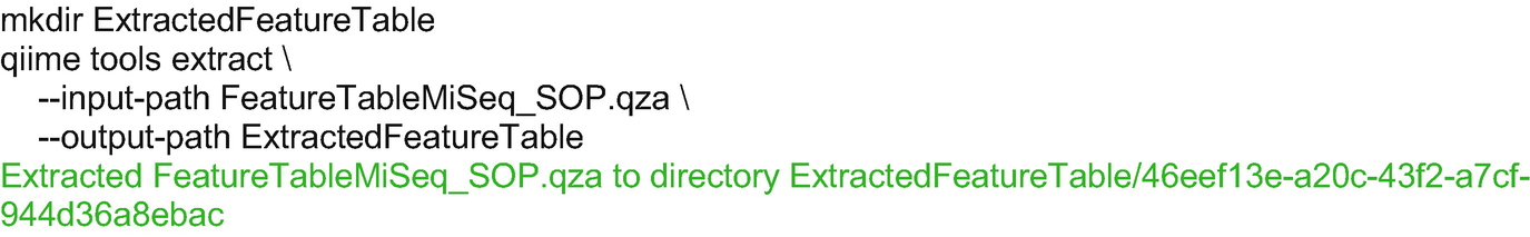
Text reads, M K D I R extracted feature table Q I I M E tools extract backward slash double hyphen input path feature table M I S E Q underscore S O P dot Q Z A backward slash double hyphen output path extracted feature table followed by a line of command.
In the above commands, we first make a directory “ExtractedFeatureTable” by the command: mkdir ExtractedFeatureTable. Then use the command: qiime tools extract to extract the data file “FeatureTableMiSeq_SOP.qza” to the created directory “ExtractedFeatureTable.” The output directory contain a new directory whose name is the artifact’s UUID (in this case, 46eef13e-a20c-43f2-a7cf-944d36a8ebac). You can check that all artifact data and metadata are stored in this directory.
3.3.2 Extract Data Using Unzip Program on macOS
Above “FeatureTableMiSeq_SOP.qza” artifact also can be extracted using unzip program as below:
The above unzip action created a new directory. The name of that directory is the UUID of the artifact being unzipped: 46eef13e-a20c-43f2-a7cf-944d36a8ebac. We can achieve a similar thing on Windows or Linux.
3.4 Filtering Data in QIIME 2
In this section, we will introduce how to filter feature tables, sequences, and distance matrices in QIIME 2.
The data that are used to illustrate the filtering functionality in QIIME 2 are FeatureTableMiSeq_SOP.qza (feature table), TaxonomyMiSeq_SOP.qza (taxonomy data), SampleMetadataMiSeq_SOP.tsv (sample metadata), “BrayCurtisDistanceMatrixMiSeq_SOP.qza” (distance matrix), and “sequences.qza” (sequence data).
Then, we put all above data into the directory just created.
3.4.1 Filter Feature Table
Filtering feature tables include filtering (i.e., removing) samples and features from a feature table. Feature tables consist of the sample axis and the feature axis. The filtering operations are generally applicable to these two axes. The filter-samples method is used to filter sample axis, whereas the filter-features method is used to filter the feature axis. Both methods are implemented in the q2-feature-table plugin. We can also use the filter-table method in the q2-taxa plugin to perform the taxonomy-based filtering: filter features from a feature table.
3.4.1.1 Total-Frequency-Based Filtering
As the name suggested, total-frequency-based filtering filters samples or features based on the frequencies that samples or features are represented in the feature table. Two usual situations are (1) filter samples when total frequency is an outlier detected in the distribution of sample frequencies; (2) set up a cut-off point or minimum total frequency and then use it as a criterion to remove samples with a total frequency less than this cut-off point.
We can use the --p-max-frequency command to filter samples and features based on the maximum total frequency. We can also combine the commands --p-min-frequency and --p-max-frequency to filter samples and features based on lower and upper limits of total frequency.

Text reads, saved feature table open square bracket frequency close square bracket to colon sample frequency filtered feature table M I S E Q underscore S O P dot Q Z A.

Text reads, saved feature table open square bracket frequency close square bracket to colon feature frequency filtered table dot Q Z A.
3.4.1.2 Contingency-Based Filtering

Text reads, saved feature table open square bracket frequency close square bracket to colon sample contingency filtered table dot Q Z A.

Text reads, saved feature table open square bracket frequency close square bracket to colon feature contingency filtered table dot Q Z A.
Similar as the total-frequency-based filtering methods, contingency-based filtering methods can use the --p-max-features and --p-max-samples parameters to filter contingent on the maximum number of features or samples. They also can optionally be used in combination with --p-min-features and --p-min-samples.
3.4.1.3 Identifier-Based Filtering
When we want to keep the specific samples or features for analysis, we can define a user-specified list of samples or features based on their identifiers (IDs) in a QIIME 2 metadata file and then use the identifier-based filtering to retain these samples or features. Since IDs will be used to identify samples or features, then a QIIME 2 metadata file that contains the IDs in the first column is required. The metadata file is used as input with the --m-metadata-file parameter.

Text reads, saved feature table open square bracket frequency close bracket to colon I D filtered table dot Q Z A.
After running the filter-samples method with the parameter --m-metadata-file SamplesToKeep.tsv, only the F3DO and F3D9 samples are retained in the IdFilteredTable.qza file.
3.4.1.4 Metadata-Based Filtering

Text reads, saved feature table open square bracket frequency close square bracket to colon male filtered table dot Q Z A.

Text reads, saved feature table open square bracket frequency close square bracket to colon time filtered table dot Q Z A.

Text reads, saved feature table open square bracket frequency close square bracket to colon early female filtered table dot Q Z A.

Text reads, saved feature table open square bracket frequency close square bracket to colon early O R female filtered table dot Q Z A.
Specifying Time='Early', Later samples would not be in the resulting table, but both Female and Male would retain in the resulting table; specifying Sex='Female', Male samples would not be in the resulting table, but both Early and Later samples would retain in the resulting table. Thus, actually evaluating OR syntax in this case would retain all of the samples. Here we just use it to illustrate the OR syntax.

Text reads, saved feature table open square bracket frequency close square bracket to colon early non-female filtered table dot Q Z A.
3.4.2 Taxonomy-Based Tables and Sequences Filtering
The filter-table method in QIIME 2’s q2-taxa plugin is designed to facilitate the process of taxonomy-based filtering, which is one of the most common types of feature-metadata-based filtering. The specific taxa can be retained or removed from a table using --p-include or p-exclude parameters, respectively.
3.4.2.1 Filter Tables Based on Taxonomy

Text reads, saved feature table open square bracket frequency close square bracket to colon feature table M I S E Q underscore S O P no mitochondria dot Q Z A.
Removing features can be done using more than one search term via listing a comma-separated search terms.

Text reads, saved feature table open square bracket frequency close square bracket to colon feature table M I S E Q underscore S O P no mitochondria no rhodobacteraceae dot Q Z A.

Text reads, saved feature table open square bracket frequency close square bracket to colon feature table M I S E Q underscore S O P with phyla dot Q Z A.

Text reads, saved feature table open square bracket frequency close square bracket to colon feature table M I S E Q underscore S O P with phyla but no mitochondria no Rhodobacteraceae dot Q Z A.
By default, QIIME 2 matches the term(s) provided for --p-include or --p-exclude if they are contained in a taxonomic annotation.
However, sometimes we want to match the terms only if they are the complete taxonomic annotation. The parameter --p-mode exact (to indicate the search should require an exact match) is designed to achieve this goal. Since the search is an exact match, the search terms are case sensitive when searching with -p-mode exact. Thus, the search term mitochondria would not return the same results as the search term Mitochondria.

Text reads, saved feature table open square bracket frequency close square bracket to colon table hyphen with hyphen phyla hyphen no hyphen mitochondria hyphen no hyphen chloroplast dot Q Z A.
In QIIME 2, we can also use qiime feature-table filter-features with the --p-where parameter to achieve the taxonomy-based filtering of tables. The qiime feature-table filter-features supports more complex filtering query than the qiime taxa filter-table filtering.
3.4.2.2 Filter Sequences Based on Taxonomy

Text reads, saved feature table open square bracket frequency close square bracket to colon sequences M I S E Q underscore S O P with phyla but no mitochondria no Rhodobacteraceae dot Q Z A.
For other filtering-sequences methods, we refer the reader to the q2-feature-table and q2-quality-control plugins. The q2-feature-table plugin also has a filter-seqs method, which can be used to remove sequences based on various criteria, including which features are present within a feature table. The q2-quality-control plugin has an exclude-seqs action, which can be used for filtering sequences based on alignment to a set of reference sequences or primers.
3.4.3 Filter Distance Matrices
The q2-diversity plugin provides the filter-distance-matrix method to filter (i.e., remove) samples from a distance matrix. It works the same way as filtering feature tables by identifiers or sample metadata.
3.4.3.1 Filtering Distance Matrix Based on Identifiers

Text reads, saved distance matrix to colon female filtered Bray Curtis distance matrix dot Q Z A.
3.4.3.2 Filter Distance Matrix Based on Sample Metadata

Text reads, saved distance matrix to colon female filtered Bray Curtis distance matrix dot Q Z A.
3.5 Introducing QIIME 2 View
QIIME 2 View (https://view.qiime2.org) is designed to allow the user to use the browser to directly open and read .qza and .qzv files that are archived on the user’s computer. Thus, it facilitates sharing the visualizations generated in QIIME 2 with a collaborator who can explore the results interactively without having QIIME 2 installed. To use QIIME 2 View, simply open it with qiime tools view or https://view.qiime2.org/ and then drag the .qza and .qzv files to the area of QIIME 2 View.
3.6 Communicating Between QIIME 2 and R
To use QIIME 2 and R integratively, some communicating tools to link them have been developed. Here, we first introduce the qiime2R package and then describe how to prepare a feature table and metadata table in R and import them into QIIME 2.
3.6.1 Export QIIME 2 Artifacts into R Using qiime2R Package
As we reviewed in Chap. 1 and so far covered in this chapter, QIIME 2 artifact is a crucial and novel concept in QIIME 2. As a method for storing the inputs and outputs for QIIME 2 as well as associated metadata and provenance information about how the object was formed, QIIME 2 artifact file in reality is a compressed directory with an intuitive structure, which has the extension of .qza. Thus QIIME 2 artifact facilitates the data storage and delivery. Although QIIME 2 equips the export tool to export QIIME 2 artifact such as exporting feature table and sequences from the artifact, however, it does not mean it is easy to import to R for the R users.
The qiime2R package was developed for importing QIIME 2 artifacts directly into R (current version 0.99.6, March 2022). The package has two important usages: (1) the read_qza() function and (2) the qza_to_phyloseq() wrapper. By using the read_qza() function, the artifact can be easily obtained into R without discarding any of the associated data. The qza_to_phyloseq() wrapper can be used to generate a phyloseq object, which is very useful when you use the phyloseq package to further analyze data. We briefly introduce these two functions below.
We continue to use the data from Example 3.9 to illustrate the qiime2R package.
3.6.1.1 Read a .qza File
3.6.1.2 Create a phyloseq Object
3.6.2 Prepare Feature Table and Metadata in R and Import into QIIME 2
When using QIIME 2 to analyze microbiome data, probably most artifacts already have been generated from a count table. However, when using R for data analysis, an artifact may be not available. In this section, we demonstrate how to generate an artifact from a count table and then import this artifact into QIIME 2. We also demonstrate how to import metadata with an appropriate format into QIIME 2.
In Example 3.4, we used the sequences data from QTRT1 (Zhang et al. 2020) to demonstrate how to import BIOM sequences data file into QIIME 2. Here, we use this dataset to illustrate how to first generate feature table and metadata table and then import an artifact and metadata into QIIME 2.
Step 1: Generate feature table in R or RStudio.
Step 2: Generate metadata table in R or RStudio.
Step 3: Convert feature table into OTU table with biom2.0 format.
Step 4: Import biom2.0 format OTU table into qiime 2.

Text reads, imported feature underscore table underscore genus underscore Q T R T 1 dot H D F 5 as B I O M V 210 format to feature underscore table underscore genus underscore Q T R T 1 dot Q Z A.
After both feature table and metadata are imported into QIIME 2, we can use them to analyze in QIIME 2.
3.7 Summary
This chapter demonstrated some basic data processing procedures in QIIME 2 with real microbiome datasets. First, importing FASTA and FASTQ format data as well as importing feature table and phylogenetic trees were described and illustrated. Then, BIOM format and Newick tree format were described and exporting feature table and exporting rooted and unrooted phylogenetic trees were illustrated. Next, two ways of extracting data from QIIME 2 archives, using the QIIME tools export command and using Unzip program on macOS, were illustrated. Followed that various filtering data methods including filtering feature table, taxonomy-based tables, and sequences filtering as well as filtering distance matrices were demonstrated. QIIME 2 View was also introduced. Finally, two ways of communicating between QIIME 2 and R were introduced and illustrated: exporting QIIME 2 artifacts into R using qiime2R package and preparing feature table and metadata in R and then importing them into QIIME 2. In Chap. 4, we will introduce building feature table and feature representative sequences from raw reads in QIIME 2.