5. Assigning Taxonomy, Building Phylogenetic Tree

5.1.1 Bioinformatics Tools and Reference Databases

Various bioinformatics tools are available for analysis of 16S rRNA gene amplicon sequencing data (Plummer et al. 2015; Nilakanta et al. 2014). Among these software, the most widely used are QIIME (Caporaso et al. 2010) and its extension of QIIME 2 (Bolyen et al. 2019), and DADA2 (Callahan 2021). In Chap. 4, we used DADA2 via QIIME 2 to generate feature frequency table and its representative sequence data table which contains the denoised sequences.

Taxonomic classification is performed after the sequences pass the filtering process, which is typically searched against a known reference taxonomy classifier at a pre-determined threshold. Most classifiers including the Ribosomal Database Project (RDP) (Cole et al. 2005), Greengenes (DeSantis et al. 2006), SILVA 16S rRNA gene database (Yilmaz et al. 2014), the UNITE database (Kõljalg et al. 2013), the National Center for Biotechnology Information (NCBI) (Federhen 2011), and EzBioCloud (Yoon et al. 2017) are publicly available. When performing taxonomic classification, we should use the frequently updated databases to avoid mapping the sequences to obsolete taxonomy names.

Currently the most often used reference databases for 16S taxonomy assignment are Silva (Quast et al. 2013), RDP (Cole et al. 2005; Maidak et al. 2000), NCBI (Federhen 2011; Geer et al. 2010), and Greengenes (McDonald et al. 2012).

SILVA (from Latin silva, forest) (Pruesse et al. 2007) is a comprehensive online resource providing quality controlled databases of aligned rRNA sequences data for all three domains of life (Bacteria, Archaea, and Eukarya) (Pruesse et al. 2012). The SILVA database is based on phylogenies for small subunit rRNAs (16S and 18S), and manually curates its taxonomic rank assignment (Yilmaz et al. 2014). Other pipelines, such as QIIME 2, DADA2, and mothur (Schloss et al. 2009), use the SILVA 16S rRNA gene reference database (Plummer et al. 2015).

Like SILVA, RDP database (Cole et al. 2005) also provides the aligned and annotated rRNA gene sequences for all three domains of life (Bacteria, Archaea, and Eukarya) and a phylogenetically consistent taxonomic framework for these data. The RDP database obtains bacterial rRNA sequences from the International Nucleotide Sequence Databases (INSD: GenBank/EMBL/DDBJ) on a monthly basis (Nakamura et al. 2012). As a Bayesian classifier, the RDP Classifier can rapidly and accurately classify bacterial 16S rRNA sequences into the new higher-order with the majority of classifications (98%) having high estimated confidence (≥95%) and high accuracy (98%) (Wang et al. 2007). RDP provides taxonomic assignments from domain to genus (Wang et al. 2007), and thus these collected 16S sequences in RDP database have not all been assigned to species level taxonomic names.

The NCBI Taxonomy project began in 1991. NCBI taxonomy database (Federhen 2011; Geer et al. 2010) is the standard nomenclature and classification repository for the International Nucleotide Sequence Database Collaboration (INSDC), comprising the GenBank (Benson et al. 2013), the European Nucleotide Archive (ENA) (EMBL) (Leinonen et al. 2011), and the DNA DataBank of Japan (DDBJ) (Mashima et al. 2017) databases (Federhen 2011). It contains all organism names and taxonomic lineages for each of the sequences associated with submissions to the NCBI global database and is manually curated to maintain a phylogenetic taxonomy for the source organisms represented in the sequence databases (Federhen 2011).

Greengenes (McDonald et al. 2012; DeSantis et al. 2006) is a chimera-check 16S rRNA gene database that has Bacteria and Archaea sequences. It provides chimera screening, standard alignment, and taxonomic classification using multiple published taxonomies. Most of the sequences in Greengenes are retrieved from NCBI database (DeSantis et al. 2006). Greengenes taxonomic classification has been improved by explicit ranks for ecological and evolutionary analyses of bacteria and archaea (McDonald et al. 2012): (1) In Greengenes a “taxonomy to tree” approach has been used for transferring group names from an existing taxonomy to a tree topology, and applied to the Greengenes, NCBI, and cyanoDB (Cyanobacteria only) taxonomies to a de novo tree sequences (McDonald et al. 2012). Reference phylogenies provide the crucial information for a taxonomic framework in interpreting marker gene and metagenomic surveys, and help to reveal novel species remarkably. (2) Explicit rank information provided by the NCBI taxonomy has been incorporated to group names for better user orientation and classification consistency and hence significantly improved the classification of the sequences in the merged taxonomy (McDonald et al. 2012). In summary, Greengenes is a dedicated full-length 16S rRNA gene database providing a curated taxonomy based on de novo tree inference. The database is used for closed-reference OTU clustering. Reads are clustered against this reference database. It has been wrapped in QIIME 1 and QIIME 2.

However, as reviewed in Chap. 4, the OTU method clustering sequences with a fixed 97% similarity threshold might avoid fine-scale variation among sequences (Rosen et al. 2012). OTUs are not species, and hence OTU method often eliminates biological information of the data, and the construction of OTUs is not necessitated by amplicon errors (Callahan et al. 2016). Thus, DADA2 uses an alternative error-modeling approach for denoising and clustering amplicons. This may be the reason that the source of GreenGenes database will no longer be maintained in DADA2 because it is deprecated (see Table 5.2). For clustering sequences into OTUs, the reader is referred to Chap. 6.

There are a variety of databases available; QIIME 2 and DADA2 have formatted and maintained most often used taxonomic reference databases.

5.1.2 QIIME 2-Formatted and Maintained Taxonomic Reference Databases

5.1.3 DADA2-Formatted and Maintained Taxonomic Reference Databases

DADA2 formatted 16S rRNA gene sequences for both bacteria and archaea (Alishum 2019). DADA2 collated and formatted two combined bacterial and archaeal 16S rRNA gene sequence databases (RefSeq+RDP and Genome Taxonomy Database (GTDB)) and used various sources for assigning taxonomy. DADA2 categorizes the 16S databases into Maintained and Contributed. DADA2 maintains reference fastas for the three most common 16S databases: Silva, RDP, and GreenGenes. It also maintains the General Fasta releases of the UNITE project for ITS taxonomic assignment. DADA2 also makes formatted versions of other databases available as “contributed.”

DADA2 created the dada2-compatible training fastas from the Silva NR99 and taxonomy files, the RDP trainset 16 and release 11.5 database, and the GreenGenes 13.8 OTUs clustered at 97%.

We summarize the DADA2-formatted and maintained taxonomic reference databases into Table 5.2 (Callahan 2021). When the reader uses these databases in Table 5.2, please check the updating from DADA2 and cite DADA2 and the original databases.

Table 5.2

DADA2-formatted and maintained taxonomic reference databases

Category	Database name	Description
Maintained databases	Silva (16S/18S rRNA) (Bokulich et al. 2021):   A list of database names. 1. Silva version 138.1 - updated March 10, 2021. 2. Silva version 132. 3. Silva version 128. 4. Silva version 123.	Like Silva version 138, the DADA2-formatted reference fastas are optimized for classification of Bacteria and Archaea, and are not suitable for classifying Eukaryotes
	RDP (Cole et al. 2005):   A list of database names. 1. R D P trainset 18. 2. R D P trainset 16. 3. R D P trainset 14.
	UNITE (fungal ITS) (Põlme et al. 2020):   A database name, U N I T E open parenthesis use the general fasta releases close parenthesis.
	Greengenes (16S rRNA) (DeSantis et al. 2006; McDonald et al. 2012; Callahan 2016):   A database name, Green genes version 13.8.	DADA2 will no longer maintain the source GreenGenes database because it is deprecated
Contributed databases	RefSeq + RDP (NCBI RefSeq 16S rRNA database supplemented by RDP) (Alishum 2019):   A list of database names. 1. Reference files formatted for assign Taxonomy. 2. Reference files formatted for assign species.	DADA2 compiled this database on May 14, 2018, from predominantly the NCBI RefSeq 16S rRNA database (https://​www.​ncbi.​nlm.​nih.​gov/​refseq/​targetedloci/​16S_​process/​) and was supplemented with extra sequences from the RDP database (https://​rdp.​cme.​msu.​edu/​misc/​resources.​jsp) This database contains 14676 bacterial and 660 archaea full 16S rRNA gene sequences
	GTDB (Genome Taxonomy Database) (Alishum 2019):   A database name, G T D B Version 202 colon Genome Taxonomy Database. Version 86 for assign taxonomy and assign species.	DADA2 downloaded this database from (http://​gtdb.​ecogenomic.​org/​downloads) on November 20, 2018 DADA2 formatted GTDB this reference sequence set which contains 20486 bacteria and 1073 archaea full 16S rRNA gene sequences
	Human InTestinal 16S rRNA (Diener 2016; Ritari et al. 2015):   A database name, Hit D B version 1.	HITdb is a reference taxonomy for Human Intestinal 16S rRNA genes as described in Ritari et al. (2015) HITdb v1.00 for Dada2 is converted version to be used with dada2 HITdb is specific for intestinal samples; thus it might lead to arbitrarily wrong results for non-intestinal samples
	RDP fungi LSU (Czaplicki 2017):   A database name, R D P fungi L S U trainset 11.	RDP LSU taxonomic training data was formatted for DADA2 (trainingset 11)
	SILVA v128 and v132 dada2 formatted 18s “train sets” (Morien and Parfrey 2018):   A database name, Silva Eukaryotic 18 S, v 132 and v 128.	These are species-level taxonomy classification training sets for the assignTaxonomy () function in DADA2 The v132 and v128 training sets include every Eukaryotic organism from SILVA’s v132 and v128 databases, respectively, clustered at 99% similarity It also includes corrected species labels for the Blastocystis clade, and includes 37 Entamoeba sequences sourced from GenBank not present in the original v128 db The v128 training set is modified specifically to allow for better species-level assignments for those two clades in mammalian gut microbiome studies
	nifHdada2: v1.1.0 (Moynihan 2020):   A database name, n i f H A R B, version 1.	This is the new reference sequences added to database
	pr2database(https://github.com/pr2database/pr2database/releases):   A database name, P R2 version 4.7.2 plus.	The provided latest PR2 version 4.14.0 is a single SSU database that contains sequences for:   18S rRNA from nuclear and nucleomorph, 16S rRNA from plastid, apicoplast, chromatophore, Mitochondrion, as well as 16S rRNA from a small selection of bacteria DADA2 note: PR2 has different taxLevels than the DADA2 default. When assigning taxonomy against PR2, use the following: assignTaxonomy(..., taxLevels = c("Kingdom","Supergroup","Division","Class","Order","Family","Genus","Species")). There are many contributors and references for this database (https://​github.​com/​pr2database/​pr2database/​releases)

5.1.4 Introduction to q2-Feature-Classifier

We may choose to train our classifiers using a suitable method, such as using q2-feature-classifier protocol that is available in QIIME 2 (Bokulich et al. 2018). The q2-feature-classifier is a QIIME 2 plugin for taxonomy classification of marker-gene sequences. It contains several novel machine-learning and alignment-based methods including a scikit-learn naïve Bayes machine-learning classifier, and alignment-based taxonomy consensus methods based on VSEARCH, and BLAST+ for classification of bacterial 16S rRNA and fungal ITS (internal transcribed spacer) marker-gene amplicon sequence data, which were evaluated as match or outperform the species-level accuracy of other commonly used methods designed for classification of marker gene sequences (Bokulich et al. 2018).

The q2-sample-classifier plugin employs scikit-learn (Pedregosa et al. 2011) for supervised learning (SL) to classify sequence and feature selection algorithms. The classify-sklearn method is a pre-fitted sklearn-based taxonomy classifier for implementing scikit-learn machine learning algorithms, while maintaining an easy-to-use interface tightly integrated with the Python language with several distinctive features including (1) it is distributed under the BSD (Berkeley Source Distribution) license; thus it has low restriction and requirement for using the distribution of many free and open source software; (2) it incorporates compiled code for efficiency; (3) it depends only on numpy and scipy to facilitate easy distribution; and (4) it focuses on imperative programming (Pedregosa et al. 2011).

The current improvement of methods for sequencing is capable to differentiate single nucleotide base: Amplicon Sequence Variants (ASVs), or sub-OTUs, which is 100% OTU. More researchers now in microbiome field including the developers of QIIME 2 recommend working with ASVs or sub-OTUs to assign taxonomy to the sequence variants, especially in 16S/18S/ITS amplicon sequencing. Thus, QIIME 2 workflow by default does not include a typical OTU picking step. Here, we follow this default direction; go directly into taxonomy assignment after using DADA2 to quality filter dataset. We will take the denoised sequences (RepSeqsMiSeq_SOP.qza) from Chap. 4 after taking denoising step, and assign taxonomy to each sequence (phylum➔ class➔…genus➔species). A trained classifier is required for this step. We can either use a reference set to train a naïve Bayes classifier and save as a QIIME 2 artifact for latter re-use, which avoids re-training the classifier between runs and saves overall running time or download a pretrained classifier.

We can use the qiime feature-classifier fit-classifier-naïve-bayes command to train a naïve Bayes classifier. If we want to use a pretrained classifier, there is a pre-trained naïve Bayes classifier artifact available in QIIME 2. This classifier was trained against Greengenes (13_8 reversion) trimmed to contain only the V4 hypervariable region and pre-clustered at 99% sequence identity (McDonald et al. 2012). We can check the QIIME 2 website (https://​docs.​qiime2.​org/​) to look for other available pre-trained artifacts.

5.1.5 Assign Taxonomy Using the q2-Feature-Classifier

Once we obtain an appropriate classifier artifact, we can use the qiime feature-classifier command to generate the taxonomic classification results. Here, we use a pretrained classifier from GreenGenes database with 99% OTUs. We download this classifier gg-13-8-99-515-806-nb-classifier.qza from the QIIME 2 website (https://​docs.​qiime2.​org/​2022.​2/​data-resources/​). To compare the denoised sequences (RepSeqsMiSeq_SOP.qza) to the GreenGenes reference database to assign taxonomy based on pairwise identity of rRNA sequences, place this classifier gg-13-8-99-515-806-nb-classifier.qza from the download in the working directory.

Please note that the scikit-learn version used to generate the reference artifact should match the current version of scikit-learn installed. Otherwise the qiime feature-classifier will not work and a plugin error message from feature-classifier will be generated. We specify the classify-sklearn method in QIIME 2 feature-classifier plugin to assign taxonomy to the representative sequences RepSeqsMiSeq_SOP.qza and save the classified taxonomy files as artifacts and name as TaxonomyMiSeq_SOP.qza.

Text reads, saved feature data open square bracket Taxonomy close bracket to colon Taxonomy M i S e q underscore S O P dot q z a.

Text reads, Saved Visualization to colon.

Since we now have three datasets: feature table, taxonomy, and sample metadata, we can use qiime taxa barplot command to create a bar plot to explore the distribution of taxonomy for each sample. Figure 5.1 can be reproduced using the following QIIME 2 commands.

# Figure 5.1:

qiime taxa barplot \

--i-table FeatureTableMiSeq_SOP.qza \

--i-taxonomy TaxonomyMiSeq_SOP.qza \

--m-metadata-file SampleMetadataMiSeq_SOP.tsv \

--o-visualization TaxaBarPlotsMiSeq_SOP.qzv

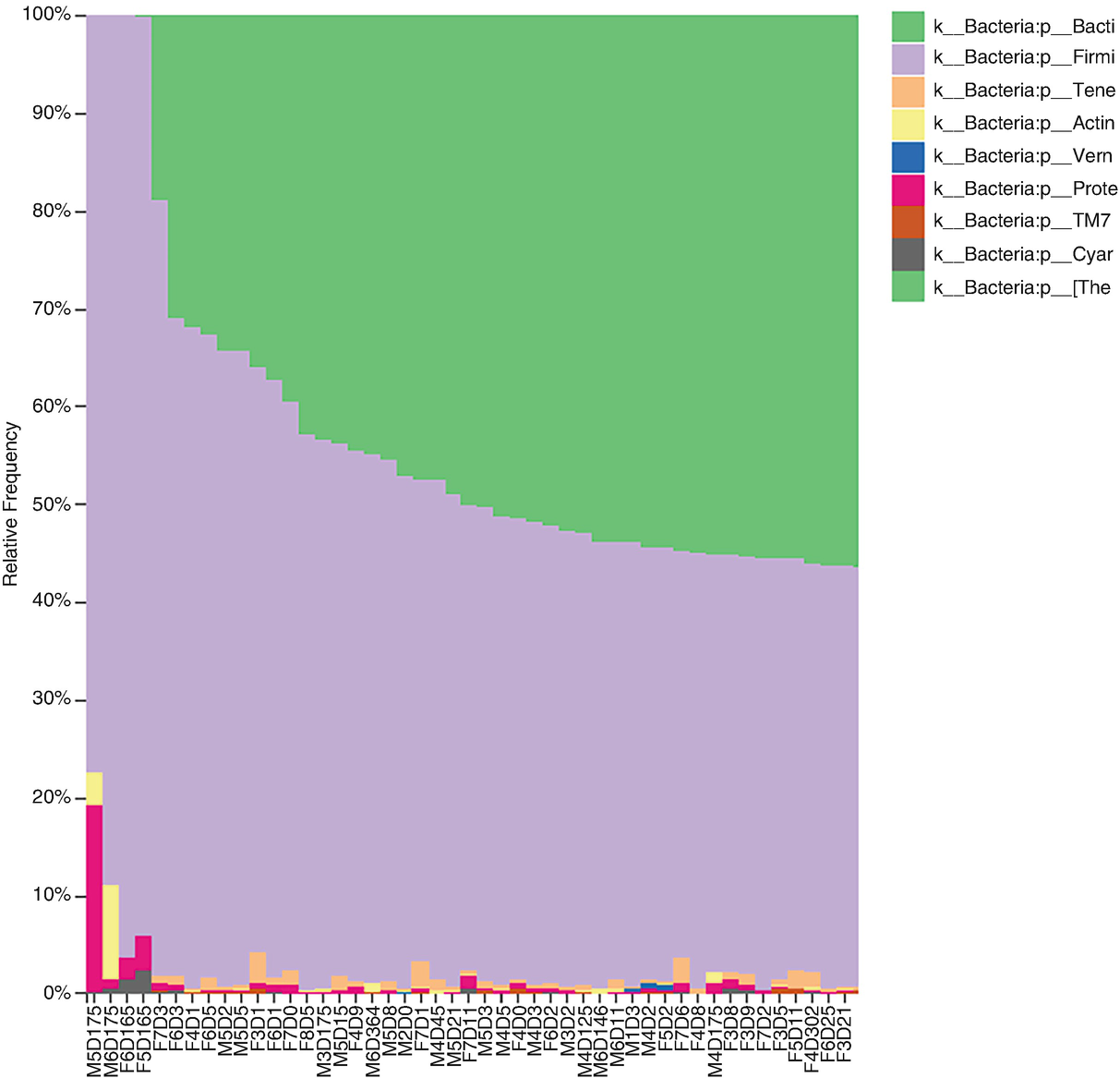
A taxa bar plot exhibits the relative frequency of the different phylum levels of bacteroidetes. The phylum levels of k underscore Bacteria colon p underscore Bacti, k underscore Bacteria colon p underscore Firmi, and k underscore Bacteria colon p underscore Tene are included.

Text reads, saved visualization to colon taxa bar plots m i s e q underscore s o p dot q z v.

We can review the visualization of the taxa bar plot in the QIIME2 viewer or use the command qiime tools view to review TaxaBarPlotsMiSeq_SOP.qzv. The generated bars can be aggregated at the desired taxonomic level, and the abundance can be sorted by a specific taxonomic group. By providing sample metadata file, we can also sort the abundance by metadata groupings. We can also interactively change color schemes, and save plots and legends in vector graphic format.

Text reads, exported feature table m i s e q underscore S O P dot q z a as B I O M V 210 d i r f m t to directory exported feature table m i s e q underscore S O P.

Then we export taxonomy information as below.

Text reads, exported taxonomy m i s e q underscore S O P dot q z a as T S V taxonomy directory format to directory exported feature table m i s e q underscore S O P.

5.1.6 Remarks on Taxonomic Classification

A number of bioinformatics tools and reference databases are available for analysis of 16S rRNA amplicon microbiome data. It was shown that taxonomy assignment often obtains different results (Balvočiūtė and Huson 2017) and especially at genus level (Sierra et al. 2020) when using different reference databases. However, currently there is no general criterion to guide for choosing appropriate bioinformatics tools and reference databases for analysis of microbiome data; and especially there are no defined criteria for data curation and validation of annotations (Sierra et al. 2020). Thus, the annotated results may be inaccurate and irreproducible, making it difficult to compare data across studies.

5.2.1 Introduction to Phylogenetic Tree

Microbiome data are encoded as a phylogenetic tree, which relates all the microbial species, containing the evolution information of the species. Thus, a phylogenetic tree is useful for incorporating biological structure (Xia 2020). Thus, one central method in computational biology is to infer evolutionary relationships or phylogenies from families of related DNA or protein sequences (Price et al. 2010). The FastTree method developed by Price et al. (2009) is to compute large minimum evolution trees with profiles instead of a distance matrix (Price et al. 2009).

5.2.2 Build a Phylogenetic Tree Using the Alignment and Phylogeny Commands

A phylogenetic tree is built in QIIME 2 via four steps: (1) multiple sequence alignment, (2) masking, (3) tree building, and (4) rooting.

MAFFT is a multiple sequence alignment program based on fast Fourier transform in evolutionary analyses of biological sequences (Katoh and Standley 2013; Katoh et al. 2002). MAFFT includes various alignment strategies as its options: progressive methods, iterative refinement methods, and structural alignment methods for RNAs. MAFFT is a similarity-based multiple sequence alignment (MSA) method, while taking evolutionary information into account because evolutionary information is useful even for similarity-based methods (Katoh and Standley 2013). QIIME wraps MAFFT’s multiple sequence alignment in the qiime alignment mafft command.

Text reads, saved feature data open bracket aligned sequence close bracket to aligned rep s e q s m i s e q underscore S O P dot q z a.

Highly variable positions could add noise to a resulting phylogenetic tree. The purpose of masking (i.e., filtering) the alignment is to remove these highly variable positions (highly gapped columns) from an alignment so that the sequences contain enough conservation to provide meaningful information. Below, we mask the uninformative positions via qiime alignment mask command.

QIIME 2 uses 40% (the default) minimum conservation as meaningful information to reproduce the mask presented in Lane (1991) via the parameter --p-min-conservation. Providing a value of 0.4 (the default), only the column that contains at least one character that is present in at least 40% of the sequences will be retained. Another default parameter used here is --p-max-gap-frequency, which is value of 1, retaining all columns regardless of gap character frequency. If a value of 0 is chosen, then retain only those columns without gap characters.

Text reads, saved feature data open bracket aligned sequence close bracket to masked aligned rep s e q s m i s e q underscore S O P dot q z a.

FastTree (Price et al. 2009, 2010) is a bioinformatic tool for inferring phylogenies for alignments. So far two versions of FastTree have been released.

Utilizing the “minimum-evolution” principle, FastTree 1 (Price et al. 2009) tries to find a topology that minimizes the amount of evolution, or the sum of the branch lengths. While via using a heuristic variant of neighbor joining method (Saitou and Nei 1987; Studier and Keppler 1988), FastTree 1 quickly finds a starting tree and using nearest-neighbor interchanges (NNIs) refines the topology (Price et al. 2010). FastTree 2 has improved its topological accuracy (the proportion of the splits in the true trees that are recovered) and 100–1,000 times faster compared to FastTree 1 and outperforms other methods including PhyML 3’s approach with default settings (NNI search) (Guindon et al. 2009, 2010), standard implementation of maximum-likelihood NNIs, minimum-evolution and parsimony methods, although not as accurate as the maximum-likelihood (ML) methods that use subtree-pruning-regrafting (SPR) moves (Price et al. 2010). The topological accuracy and outperformances are achieved by FastTree 2 mostly because FastTree 2 (1) adds minimum-evolution SPRs, (2) adds maximum likelihood NNIs, (3) uses heuristics to restrict the search for better trees, and (4) estimates a rate of evolution for each site (Price et al. 2010).

QIIME builds a phylogenetic tree based on FastTree (Price et al. 2010) via the qiime phylogeney fasttree command.

Text reads, saved phylogeny open bracket unrooted close bracket to colon unrooted tree m i s e q underscore S O P dot q z a.

By processing the FastTree method, an unrooted phylogenetic tree is generated from the masked alignment. However, some downstream analyses require a rooted tree; thus we use the longest branch to root the tree at the midpoint of the two leaves that are the furthest from one another (called “midrooting”), producing the rooted tree artifact file “RootedTreeMiSeq_SOP.qza” that can be used as input to generate phylogenetic-diversity measures.

Text reads, saved phylogeny open bracket rooted close bracket to colon rooted tree m i s e q underscore S O P dot q z a.

5.2.3 Remarks on the Taxonomic and Phylogenetic Trees

Taxonomy and phylogeny are two concepts involved in the classification of organisms. Taxonomy stems from ancient Greek taxis, meaning “arrangement,” and nomia, meaning “method.” Taxonomy is a field of classification, identification, and naming of biological organisms based on their shared characteristics of similarities and dissimilarities (Xia et al. 2018).

Classification of organisms was first introduced by the Swedish botanist Carl Linnaeus (1707–1778) (known as the father of taxonomy). He developed a system for categorization of organisms, known as Linnaean taxonomy and binomial nomenclature for categorizing and naming organisms.

Linnaeus and others ranked all living organisms into seven biological groups or levels of classification in the taxonomic hierarchy: kingdom, phylum, class, order, family, genus, and species. There are no domains in their classifications. The classification of domain was first proposed by Woese et al. in 1977 (Woese and Fox 1977; Woese et al. 1990). They added a level called “domain” above the level of kingdom. The three domains of life are Archaea, Bacteria, and Eukarya, and the five major kingdoms are monera, protista, fungi, plantae, and animalia. Thus, we can classify all living organisms into eight major hierarchical levels, from domain (the most general) to species (the most specific): domain, kingdom, phylum, class, order, family, genus, and species.

A phylogenetic tree (also called phylogeny or evolutionary tree) (Felsenstein 2004) is a branching diagram or a tree showing the evolutionary relationship of a species or a group of species with a common ancestor based upon similarities and differences in their physical or genetic characteristics.

Various ways have been developed to graphically represent the phylogenetic trees (Letunic and Bork 2006). Both taxonomy and phylogeny are important for classification of organisms. Phylogeny is important in building taxonomy. Researchers have attempted to synthesize phylogeny and taxonomy into a comprehensive tree of life (Hinchliff et al. 2015). However, taxonomy and phylogeny as well as taxonomic tree and phylogenetic tree are different. The key difference between these two pairs of concept lies in the fact that taxonomy/taxonomic tree involves naming and classifying organisms while phylogeny/phylogenetic tree involves the evolution of the species or groups of species. Taxonomy focuses on naming and classifying organisms, and hence does not reveal anything about the shared evolutionary history of organisms. In contrast, phylogeny focuses on evolutionary relationships of organisms and hence reveals the shared evolutionary history.

Additionally, as shown in above illustrating examples, their reconstructions are also different. For amplicon sequencing, the taxonomic tree is typically reconstructed when the phylogeny is not available but taxonomic annotations are available. The taxonomic tree is reconstructed from lineages extracted from regularly updated databases such as from NCBI (Federhen 2011; Geer et al. 2010) and represents the alignment from domain to species rank; as discovery of new species continues, assignment of new taxa in the taxonomic hierarchy will never end. Thus, taxonomic trees are highly polyatomic. In contrast, the phylogenetic tree is reconstructed based on the sequence divergence of taxa (of the marker-gene) (Price et al. 2010) and it encodes the common evolutionary history of the taxa. In other words, phylogenetic trees are reconstructed usually based on morphological or genetic homology to reveal the evolutionary relationships of species via comparison of anatomical traits and to reveal the ancestral genes (identify descent from an ancestral gene) via analysis of genetic differences of species. Thus, unlike taxonomic trees, phylogenetic trees are hypothetic (Dubois et al. 2021; Felsenstein 2004).

Phylogenetic classification has two main advantages over the Linnaean classification. First, phylogenetic classification reveals the evolutionary history of the organism: the important underlying biological processes that are responsible for the diversity of organisms. Second, phylogenetic classification does not attempt to “rank” organisms and hence avoids the misleading of considering different groupings with the same rank are equivalent and comparable. Actually, comparing to phylogenetic tree, taxonomic tree ignores the granular differences of the taxa belonging to the same rank. However, the advantage of phylogenies is that they do not capture similarities between taxa in terms of abundance profiles (Bichat et al. 2020).

Human microbiome is very complicated with existing genetic and evolutionary relationships among species. To understand the complexity of the human microbiome, it is important to recognize the genetic and evolutionary relationships between species. Microbiome data are encoded as the taxonomic and phylogenetic trees. Both taxonomic and phylogenetic trees play important roles in microbiome studies. As two unique features in the microbiome data, these two trees are usually used for different measures and are required by different strategies of statistical analysis.

Integrating the information of the taxonomic and phylogenetic trees into statistical analysis will increase statistical power in statistical hypothesis testing. For example, it has been believed that reference phylogenies can prove the crucial information into a taxonomic framework for interpretation of marker gene and metagenomic surveys to speed revealing novel species (McDonald et al. 2012), and leveraging the phylogenetic tree of the taxa can increase statistical power while controlling the False Discovery Rate (FDR) (Sankaran and Holmes 2014; Xiao et al. 2017).

However, the premise that the phylogenetic (or taxonomic) tree is the relevant hierarchical structure to incorporate in differential studies has been questioned in recent study; and it was showed that incorporating phylogenetic information in microbiome differential abundance analyses has no effect on detection power and FDR control (Bichat et al. 2020). Instead in this study (Bichat et al. 2020) a correlation-tree was proposed and advocated for use. A correlation-tree is a clustering tree built based on the abundance profiles of taxa across samples, in which taxa with highly correlated abundances are very close in the tree. The correlation tree is built involving three logical steps: (1) computing the pairwise correlation matrix using the Spearman correlation and excluding samples where both taxa are absent; (2) using the transformation to change the correlation matrix into a dissimilarity matrix; and (3) creating the correlation tree using hierarchical clustering with Ward linkage on this dissimilarity matrix. Branch lengths correspond to the dissimilarity cost of merging two subtrees.

The correlation tree was considered being better than the phylogenetic tree for a proxy of biological functions and increasing the detection power while with better FDR control (Bichat et al. 2020). However, it needs for evaluation by other studies and/or deserves to be further discussed and assessed whether above arguments are true and whether or not the correlation tree is more important than the phylogenetic tree in differential abundance analysis.

As reviewed the history of numerical taxonomy, we learn that early in 1950s the “taxonomic importance” was criticized by Cain (Cain 1958). Cain was not opposed to phylogeny per se, instead thought that we ought to incorporate phylogenetic information into classification when it is available and reliable. However, he recognized it was very difficult to do and in some cases classification should be purely phenotypic (Vernon 1988).